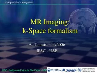
MR Imaging: k-Space formalism
860 likes | 1.38k Vues
MR Imaging: k-Space formalism. A. Tannús – 11/2006 IFSC - USP. Nobel prizes: NMR as a source of insight. 1942 (1930): Physics: I. Rabbi: Resonant method for measuring magnetic properties of atomic nuclei. 1952 (1946): Physics : F. Bloch & E. Purcell:

MR Imaging: k-Space formalism
E N D
Presentation Transcript
MR Imaging:k-Space formalism A. Tannús – 11/2006 IFSC - USP
Nobel prizes: NMR as a source of insight • 1942 (1930): Physics: I. Rabbi: • Resonant method for measuring • magnetic properties of atomic nuclei. 1952 (1946): Physics : F. Bloch & E. Purcell: Precision measurement of Nuclear Magnetism
Nobel prizes in MR 1992 (1966): Chemistry: R. Ernst: High Resolution Pulsed Magnetic Resonance - Spectroscopy. 2003 (1973): Medicine: P. Mansfield & P. C. Lauterbur Magnetic Resonance Imaging.
MRI temporal and spatial resolution Improve Improve
NMR Phenomena • Quantum Mechanical approach: • Easy for spin ½; • Gets complex when dealing with different nuclear species in a system. • Classical Approach. • Explain almost completely the development of Imaging methodologies. To QM..
Classical Approach Fundamental properties of nuclei Evolution described by an equation of a precessing rotor
Spinning Top in a gravitational field:a very bad example… “Spinning nucleus” B0 “Spinning Top” Reaction from base m = magnetic moment L=angular momentum L=angular momentum t = magnetically induced torque = - mxB0 Weight force • = torque produced by the binary forces: Weight and reaction at contact point
Macroscopic Magnetization Relaxation T1 and T2 are determined based on experimental results! (Phenomenology)
z a) B e.m.f o y x M V(t) Excitation/Detection Scheme e.m.f B1
Detected signal Induced e.m.f. FID t
Imaging Scanner Overview:Hardware Fully digital, multichannel now! Work in progress at our group Gradient Controller Master Controller X Y Z RF Controller RF Amplifier DAC Receiver Gradient Coil RF coil preamp Magnet
Other Magnet Types Permanent magnets, e.g. light weight rare earth magnets, <0.3T “H” type, transverse access “C” type, transverse access (open systems)
Other Magnet Types “H” and “C” mixed type, transverse access (open systems)
Other Magnet Types Electromagnet <0.3T
RF Coils Remember: Brf (B1) must be orthogonal toB0 !! Saddle coil allows axial access. Efficiency is low, and homogeneity is poor Field is aligned to subject; Other designs than solenoidal must be used.
z z z y y y x x x Gz Gx Gy Imaging basic principles: encoding Now that we have an NMR signal, how to get an image? By mapping the spins according to their position. How?Using their frequency/position correspondence(r) =B0(r)
A bit of history… P. C. Lauterbur - (1973) State University - New York First 2D NMR image: came from an annoyance for spectroscopists!!! Projection/Reconstructionmethod(same as in CT)
Encoding inmore than one dimension:solving the projection paradox. Magnetic field gradients add as vectors, giving a newly oriented gradient!!
Magnetic Field Gradients Now, gradients are time dependent!!
Spatially encoded frequency and phase:more than one dimension?
The 3D Image Equation!! 3D Signal 3D Image
B0 z RF Gz x Gz y e.m.f. Steps to NMR Imaging Selective excitation • Absorption line broadening • Narrow bandwidth RF pulses Only spins inside this band are excited
Gy B0 z Gz Gy x y e.m.f Principles of NMR Imaging Phase encoding Selective excitation • Absorption line broadening • Narrow bandwidth RF pulses Encoding in this dimension is done through the initial phase.
z B0 Gx x Gz y e.m.f Gy Gx Principles of NMR Imaging Frequency encoding Phase encoding Selective excitation • Absorption line broadening • Narrow bandwidth RF pulses Encoding in this dimension is done through the spatially dependent frequency.
Gz Gy Gx Principles of NMR Imaging Phase encoding Frequency encoding Selective excitation • Absorption line broadening • Narrow bandwidth RF pulses
ky p p/2 RF Gz p Gy A’’ A A’ Gx kX 0 FID ECO Gz B Signal Gy C t @ 0 Gx B’ C’ 2t tC tB tA @ B’’ C’’ Acquisition Preparation Principles of NMR Imaging Acquisition sequences and image formation : • Spin Echo ( SE ) • Spin Echo ( SE ) • Echo Planar Imaging ( EPI ) • Gradient Recalled Echo ( GRE )
k-space • k-space is the raw data space before Fourier transformation into the image • 2D image will be represented by a 2D array of data points spread throughout k-space (it could be 3D!!) • Changing the k-space trajectory will alter image contrast
k-space • k-space must be sampled in equally spaced intervals in order to allow 2D FFT. • As a consequence the image is also presented in equally spaced sampled values. • All concepts of discrete Fourier formalism applies.
Image vs. k-space data (r) S(k) k(t)= /2G(t)dt
Image vs. k-space data (r) S(k) k(t)= /2G(t)dt
Image vs. k-space data (r) S(k) k(t)= /2G(t)dt
Image vs. k-space data (r) S(k) k(t)= /2G(t)dt
Image vs. k-space data FFT (r) S(k) k(t)= /2G(t)dt
GE k-space trajectory RF G S G R G P S(t) (r) S(k) k(t)= /2G(t)dt
GE k-space trajectory RF G S G R G P S(t) -kr +kr (r) S(k) k(t)= /2G(t)dt
GE k-space trajectory RF G S G R G P S(t) -kr +kr (r) S(k) k(t)= /2G(t)dt
GE k-space trajectory +kp RF G S G R G P S(t) -kp -kr +kr (r) S(k) k(t)= /2G(t)dt
GE k-space trajectory +kp RF G S G R G P S(t) -kp -kr +kr (r) S(k) k(t)= /2G(t)dt
GE k-space trajectory +kp RF G S G R G P S(t) -kp -kr +kr (r) S(k) k(t)= /2G(t)dt
GE k-space trajectory +kp RF G S G R G P S(t) -kp -kr +kr (r) S(k) k(t)= /2G(t)dt
GE k-space trajectory +kp RF G S G R G P S(t) -kp -kr +kr (r) S(k) k(t)= /2G(t)dt
GE k-space trajectory +kp RF G S G R G P S(t) -kp -kr +kr (r) S(k) k(t)= /2G(t)dt
GE k-space trajectory +kp RF G S G R G P S(t) -kp -kr +kr (r) S(k) k(t)= /2G(t)dt
GE k-space trajectory +kp RF G S G R G P S(t) -kp -kr +kr (r) S(k) k(t)= /2G(t)dt