Download
1 / 72
720 likes | 870 Vues
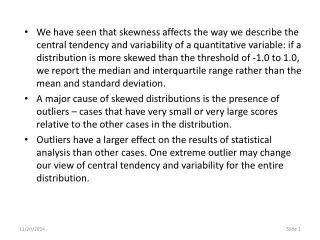
We have seen that skewness affects the way we describe the central tendency and variability of a quantitative variable: if a distribution is more skewed than the threshold of -1.0 to 1.0, we report the median and interquartile range rather than the mean and standard deviation.

E N D
We have seen that skewness affects the way we describe the central tendency and variability of a quantitative variable: if a distribution is more skewed than the threshold of -1.0 to 1.0, we report the median and interquartile range rather than the mean and standard deviation. • A major cause of skewed distributions is the presence of outliers – cases that have very small or very large scores relative to the other cases in the distribution. • Outliers have a larger effect on the results of statistical analysis than other cases. One extreme outlier may change our view of central tendency and variability for the entire distribution.
Outliers pose a dilemma for us in terms of our justification for either omitting them or retaining them in the analysis. • It is easy to remove outliers that were data entry errors. It is more difficult to defend removing outliers when the scores represent accurate data. • One response to the dilemma is to run the analysis with and without the outliers, and describe the difference. Sometimes it makes little difference and we can ignore the presence of the outliers. • Another response to the dilemma is to re-express or transform the variable and see if the outliers are eliminated. If there are no outliers using the re-expressed data, we can run the analysis with the re-expressed data and draw our conclusions based on the results for the re-expressed variables.
Two downsides to the strategy of re-expressing data are: • the skepticism of audiences who already think we massage the numbers to produce the results we want, and • the need to convert the results back to the original scale if we need to report numerical results. • In this problem set, we will use a boxplot strategy for detecting outliers and examine the use of two of the possible transformations: the square and the logarithm. • The Explore procedure in SPSS provides both the boxplot and the descriptive statistics needed to solve these problems. • In the boxplot, two types of outliers are identified by symbols: circles for outliers, and stars for extreme (or far) outliers.
A case is identified as an outlier (circle) if its value is less than or equal to the first quartile minus 1.5 times the interquartile range, or is greater than or equal to the third quartile plus 1.5 times the interquartile range. • If the case has a value less than or equal to the first quartile minus 3 times the interquartile range or greater than the third quartile plus 3 times the interquartile range, it is characterized as a far outlier (stars). • If outliers or far outliers are found for a variable, we will examine the behavior of the outliers when the variable is re-expressed by computing the logarithm of the values if the variable is skewed to the right. If the variable is negatively skewed, we will square the values and examine the effect on the outliers.
The script for this week positions the boxplot under the histogram. In this chart, we see a number of circles at the right end of the distribution. These are outliers, and there are no far outliers in this distribution. As we would expect, this distribution has a skewness problem (skewness=1.19) in the subtitle to the chart. NOTE: the horizontal axis for the boxplot approximates the axis for the histogram, but is not exact.
This distribution for this variable shows one far outlier at the extreme right of the distribution.
Some distributions will show both outliers and far outliers. Our problems will state the number of outliers, and the number of far outliers as a subset of the total number of outliers. Note that the chart shows the presence or absence of outliers, but does not necessarily provide an exact count since the outlier symbol might represent more than one case with the score.
The boxplots for some distributions will indicate that there are no outliers.
When we re-express the values for the variable on a logarithmic scale, the boxplot does not indicate that there are any outliers. The boxplot for the distribution for this variable shows several outliers at the right end of the distribution. When the variable is positively skewed, the data values are re-expressed on the logarithmic scale.
If we re-express the data values using the wrong transformation, we actually increase the problem of outliers. The distribution was positively skewed, and we squared the data values, rather than converting to a log scale, resulting in more outliers.
The boxplot for the distribution for this variable shows several outliers at the low end of the scale. Since this variable is skewed to the left, we will re-express the data values as squares. The boxplot of the squared values indicates that there are not outliers for the re-expressed data values.
If we re-express the data values using the wrong transformation, we actually increase the problem of outliers. The distribution was negatively skewed, and we applied a log transformation rather than the square transformation, resulting in more outliers.
Re-expressing the data values does not always remedy the problem of outliers. In the chart to the right, the logarithmic transformation appears to have had little impact.
Some variables have outliers at both ends of the distribution. The outliers at one end may offset the skewness in the other tail, but kurtosis will become a problem. Neither the logarithmic nor the square transformation will remedy this distribution because each re-expression works on only one tail of the distribution.
Re-expression changes the measuring scale for the variable by altering the distance between the values. All of the lines below represent the numbers 1 to 10, on a decimal, logarithmic, and squared scale. • On our familiar decimal measuring scale, the distance between numbers is the same for all numbers. • On a logarithmic scale, the distance between the numbers decreases as the numbers get larger • On a square scale, the distance between the numbers decreases as the values get smaller. • All of the dots represent the same sequence of values from 1 to 10 on different measuring scales.
The logarithmic transformation works by stretching the scale at the left end of the distribution and compressing the scale at the right end of the distribution. • As shown in the diagram below, the numbers 1 to 5 (red dots) are converted to their log equivalents (blue dots). The distance between the log points decreases as the values increase. The distance between the log of 4 and the log of 5 is less than the distance between the log of 1 and log of 2.
Positive skewing is reduced because the distance between consecutive numbers on the decimal scale decreases as the size of the decimal number increases. • For example, the difference between the log of 2 and the log of 3 is 0.176, larger than the difference between the log of 4 and log of 5, which is 0.097.
The square transformation works by compressing the scale at the left end of the distribution and stretching the scale at the right end of the distribution. • As shown in the diagram below, the numbers 1 to 5 (red dots) are converted to their squared equivalents (blue dots). The distance between the squared points increases as the values increase. The distance between the square of 4 and the square of 5 is larger than the distance between the square of 1 and square of 2.
Negative skewing is reduced because the distance between consecutive numbers on the decimal scale increases as the size of the decimal number increases. • For example, the difference between the square of 2 and the square of 3 is 5.0, less than the difference between the square of 4 and square of 5, which is 9.0.
As long as we can reverse the transformation and get back to the original values, the transformations are legitimate. • To make certain we can get back to the original values, we must make certain the numbers on all scales are mathematically defined as real numbers. Not all numbers are defined, such as the logarithm of 0 and the square root of negative numbers. • To make certain we do not do a transformation we cannot work backwards, we may need to add a constant to each number. If numbers are negative, we add the amount of the smallest value to each number. If the smallest value in the distribution is 0, we add 1 to each score in the distribution. • Since we are starting out with transformations, the problem statement will tell you if you need to add a numeric constant when doing the transformations.
The introductory statement in the question indicates: • The data set to use (2001WorldFactBook) • The task to accomplish (checking for outliers) • The SPSS procedure to use (Explore) • The variable to use in the analysis: HIV-AIDS adult prevalence rate [hivaids]
These problem also contain a second paragraph of instructions that provide the formulas to use if our examination of outliers requires us to re-express or transform the variable.
The first statement concerns the number of valid and missing cases. To answer this question, we produce the descriptive statistics using the SPSS Explore procedure.
To compute the descriptive statistics and charts that we need to check for outliers, select the Descriptive Statistics > Explore command from the Analyze menu.
Move the variable for the analysis hivaids to the Dependent List list box.. Click on the Statistics button to select optional statistics.
The check box for Descriptives is already marked by default. Mark the Percentiles check box. This will provided the upper and lower bounds for the interquartile range. Click on Continue button to close the dialog box. While there is a check box for Outliers, it lists the five largest scores and the five smallest scores, but does not tell us whether or not they are really outliers.
Next, we click on the Plots button to obtain visual evidence of the presence of outliers in the distribution.
We accept the default for the Box plot, which provides us the output we need even though we are not using factor levels in this problem. We click on the Continue button to close the Plots dialog. We accept the default Stem-and-Leaf plot, and mark the check box for a Histogram as well.
After returning to the Explore dialog box, click on the OK button to produce the output.
The SPSS output provides us with the answer to the question on sample size. The 'Case Processing Summary' in the SPSS output showed the total number of valid cases to be 162 and the number of missing cases to be 56.
The 'Case Processing Summary' in the SPSS output showed the total number of valid cases to be 162 and the number of missing cases to be 56. Click on the check box to mark the statement as correct.
The next two statements focus on the median and interquartile range as the center and spread of the data. We are using the median and interquartile range because we are using the box plot strategy for identifying outliers. The median and interquartile range are key measures of box plots.
We use the table of descriptive statistics to obtain the value for the median: .2000 for this variable. However, we do not use the table of descriptive statistics for the value of the interquartile range because this is not the value used in the box plot. The value used in the box plot is based on “Tukey’s hinges” which use a slightly different calculation for the first and third quartile, which may make a difference in the value for the interquartile range.
The value for the first quartile (the 25th percentile) is 0.050. The value for the third quartile (the 75th percentile) is 2.010. The interquartile range is the difference between the two: 1.96 (2.010 – 0.050 = 1.96). Note that the 75th percentile using the default weighted average calculation is slightly different (2.0150) from the 75th percentile calculated with Tukey’s Hinges.
From the SPSS output, we obtained a value of 0.20 for the median and 1.96 for the interquartile range. We mark the first check box in the pair as the correct answer.
The next pair of statements asks us to identify the direction of the skewing in the distribution of the variable. Outliers almost always skew the distribution. The direction of the skewness is critical because it dictates which function we choose to re-express or transform the data.
The skewness for the distribution of "HIV-AIDS adult prevalence rate" [hivaids] is 3.19. Since this is greater than zero, we characterize it as positive skewing, or skewing to the right. When the distribution is skewed to the right, the text recommends re-expressing the data as logarithms, square roots, or reciprocals. We will use logarithms in these problems. When the distribution is skewed to the left, the text recommends re-expressing the data as squares.
The skewness for the distribution of "HIV-AIDS adult prevalence rate" [hivaids] is 3.19. Since this is greater than zero, we characterize it as positive skewing or skewing to the right. We mark the check box for the first statement as the correct response.
The next pair of statements asks us to identify how many outliers there are in the distribution, either that there are no outliers or that there are a specific number of outliers and far outliers.
The box plot provides us with the first evidence of outliers. The circles and asterisks above the whiskers of the box plot attest to the presence of outliers. In the terminology of the text, the circles are outliers, and the asterisks are far outliers.
If the variable does not have outliers, neither circles nor asterisks will appear in the box plot. This is a box plot for the variable Population below poverty line from the same data set.
While the box plot makes it obvious that there are outliers in this distribution, it is not possible to obtain the exact number because the points overlap and because a single circle or star may represent more than one case with that value.
The presence of outliers is also seen in the histogram of the distribution. However, it also does not make it easy to determine the exact number.
Our first task is to compute the values that would let us determine whether or not a case is an outlier. • The value for the first quartile (the 25th percentile) is 0.050. The value for the third quartile (the 75th percentile) is 2.010. The interquartile range is the difference between the two: 1.96 (2.010 – 0.050 = 1.96). • To be characterized as an outlier, a case would have to have: • a value less than or equal to -2.89 (Q1 - 1.5 x IQR = 0.05 - 1.5 x 1.96 = -2.89) • or • a value greater than or equal to 4.95 (Q3 + 1.5 x IQR = 2.01 + 1.5 x 1.96 = 4.95)
Our second task is to compute the values that would let us determine whether or not a case is a far outlier. • The value for the first quartile (the 25th percentile) is 0.050. The value for the third quartile (the 75th percentile) is 2.010. The interquartile range is the difference between the two: 1.96 (2.010 – 0.050 = 1.96). • To be characterized as a far outlier in the distribution of "HIV-AIDS adult prevalence rate" [hivaids], a case would have to have • a value less than or equal to -5.83 (Q1 - 3 x IQR = 0.05 - 3 x 1.96 = -5.83) • or • a value greater than or equal to 7.89 (Q3 + 3 x IQR = 2.01 + 3 x 1.96 = 7.89) The calculations may produce values that do not exist in the data set, e.g. -5.83. Since there can be no outliers at that value or smaller, it does not have any impact on our solution.
We sort the cases in ascending order by the variable we are studying, so we can count the number of cases that fall in the outlier region. Click the right mouse button on the column header for hivaids, and select Sort Ascending from the pop-up menu.
The entries at the top of sorted column are missing values, indicated by the periods in the cells. The lower bounds for both outliers and far outliers were negative numbers (-2.89 and -5.83). Since all of the values for hivaids are positive numbers there are no outliers in the lower range of values.
The upper bound for outliers was 4.95. After locating in the sorted column, we count the number of values greater than or equal to 4.95., as shown in the red border. There are 25 outliers. The upper bound for far outliers was 7.89, outlined with the blue border. There are 18 far outliers.
We counted 25 outliers and 18 far outliers in the data editor for hivaids. We mark the second check box in the pair which concurs with our finding.
The first statement in the next pair asks about the impact of re-expressing or transforming the data as logarithms. It predicts that the logarithmic transformation will eliminate both outliers and far outliers.