Download
1 / 32
410 likes | 712 Vues
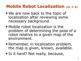
Mobile Robot Localization (ch. 7). Mobile robot localization is the problem of determining the pose of a robot relative to a given map of the environment. Because, Unfortunately, the pose of a robot can not be sensed directly, at least for now. The pose has to be inferred from data.

E N D
Mobile Robot Localization (ch. 7) • Mobile robot localization is the problem of determining the pose of a robot relative to a given map of the environment. Because, • Unfortunately, the pose of a robot can not be sensed directly, at least for now. The pose has to be inferred from data. • A single sensor measurement is enough? • The importance of localization in robotics. • Mobile robot localization can be seen as a problem of coordinate transformation. (One point of view.)
Mobile Robot Localization • Localization techniques have been developed for a broad set of map representations. • Feature based maps, location based maps, occupancy grid maps, etc. (what exactly are they?) (See figure 7.2) • (You can probably guess What is the mapping problem?) • Remember, in localization problem, the map is given, known, available. • Is it hard? Not really, because,
Mobile Robot Localization • Most localization algorithms are variants of Bayes filter algorithm. • Different representation of maps, sensor models, motion model, etc lead to different variant. • Here is the agenda.
Mobile Robot Localization • We want to know different kinds of maps. • We want to know different kinds of localization problems. • We want to know how to solve localization problems, during which process, we also want to know how to get sensor model, motion model, etc.
Mobile Robot Localization(We want to know different kinds of maps. ) Different kinds of maps. At a glance, …. feature-based, location-based, metric, topological map, occupancy grid map, etc. see figure 7.2 • http://www.cs.cmu.edu/afs/cs/project/jair/pub/volume11/fox99a-html/node23.html
Mobile Robot Localization – A Taxonomy (We want to know different kinds of localization problems.) • Different kinds of Localization problems. • A taxonomy in 4 dimensions • Local versus Global (initial knowledge) • Static versus Dynamic (environment) • Passive versus active (control of robots) • Single robot or multi-robot
Mobile Robot Localization • Solved already, the Bayes filter algorithm. How? • The straightforward application of Bayes filters to the localization problem is called Markov localization. • Here is the algorithm (abstract?)
Mobile Robot Localization • Algorithm Bayes_filter ( ) • for all do • endfor • return
Mobile Robot Localization • Algorithm Markov Locatlization ( ) • for all do • endfor • return The Markov Localization algorithm addresses the global localization problem, the position tracking problem, and the kidnapped robot problem in static environment.
Mobile Robot Localization • Revisit Figure 7.5 to see how Markov localization algorithm in working. • The algorithm Markov Localization is still very abstract. To put it in work (eg. your project), we need a lot of more background knowledge to realize motion model, sensor model, etc…. • We start with Guassian Filter (also called Kalman filter)
Bayes Filter Implementations (1) Kalman Filter (Gaussian filters) (back to Ch.3)
Kalman Filter • The discovery of KF --- one of the greatest discoveries in the history of statistical estimation theory and possibly the greatest in the 21th century. • Has been used in many application areas ever since Richard Kalman discovered the idea in 1960. • The KF has made it possible for humans to do things that would not have been possible without it. • In modern technology, KFs have become as indispensable as silicon chips.
Bayes Filter Reminder • Prediction • Correction
m Univariate -s s m Multivariate Gaussians
Multivariate Gaussians • We stay in the “Gaussian world” as long as we start with Gaussians and perform only linear transformations. • Review your probability textbook http://en.wikipedia.org/wiki/Multivariate_normal_distribution
Kalman Filter Estimates the state x of a discrete-time controlled process that is governed by the linear stochastic difference equation with a measurement
Components of a Kalman Filter Matrix (nxn) that describes how the state evolves from t-1 to t without controls or noise. Matrix (nxl) that describes how the control ut changes the state from t-1 to t. Matrix (kxn) that describes how to map the state xt to an observation zt. Random variables representing the process and measurement noise that are assumed to be independent and normally distributed with covariance Rt and Qt respectively.
Kalman Filter Algorithm • Algorithm Kalman_filter( mt-1,St-1, ut, zt): • Prediction: • Correction: • Returnmt,St
Linear Gaussian Systems: Initialization • Initial belief is normally distributed:
Linear Gaussian Systems: Dynamics • Dynamics are linear function of state and control plus additive noise:
Linear Gaussian Systems: Observations • Observations are linear function of state plus additive noise:
Linear Gaussian Systems: Observations See page 45-54 for mathematical derivation.
Prediction The Prediction-Correction-Cycle
Correction The Prediction-Correction-Cycle
Prediction Correction The Prediction-Correction-Cycle
Kalman Filter Summary • Highly efficient: Polynomial in measurement dimensionality k and state dimensionality n: O(k2.376 + n2) • Optimal for linear Gaussian systems! • However, most robotics systems are nonlinear, unfortunately!