Download
1 / 11
110 likes | 253 Vues
This study explores the dynamic pathways of combustion byproducts through flow reactor experiments, applying quantum mechanical methods to understand molecular properties and reaction dynamics. Additionally, ambient air quality data is analyzed for epidemiological studies, focusing on criteria pollutants like PM and NO2. Statistical models assess measurement errors and spatial variations across monitoring sites, providing insights into source attribution and regional transport effects. The findings emphasize the importance of precise data handling to account for local and regional influences on air quality.

E N D
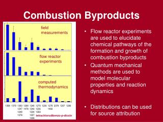
Combustion Byproducts field measurements • Flow reactor experiments are used to elucidate chemical pathways of the formation and growth of combustion byproducts • Quantum mechanical methods are used to model molecular properties and reaction dynamics • Distributions can be used for source attribution flow reactor experiments computed thermodynamics tetrachlorodibenzo-p-dioxin
Air Quality Data Analyses for Epi Studies • Criteria pollutant analyses • most representative value • error and spatial variation • PM component analyses • air quality modeling • source apportionment modeling
normalized values • x’ = (x-x)/x • ’ = 0 • ’ = 1 = 1 = 0
error and spatial variation differences between two sites {(x’-y’)/2}: = 0 spatial sd = {(1-R)/2}½ averages of two sites over time {(x’+y’)/2}: = 0 temporal sd = {(1+R)/2}½ differences due to error and spatial variation: • measurement error co-located instruments • instrument, laboratory (PM), and human • spatial variation • local sources nearby monitoring sites • regional transport/meteorology entire study area = 0
example: NO2 – monitoring sites 1-hr correlation, R GT-JS 0.59 GT-SD 0.67 GT-Tu 0.76 GT-CO 0.44 GT-Yo 0.05 JS-SD 0.51 JS-Tu 0.57 JS-Co 0.38 Tu Yo GT JS SD Co 130 km x 130 km
variogram spatial sd / temporal sd R {(1-R)/(1+R)}½ 1 0 0 1 -1 1 regional effects {(1-R)/(1+R)}½ local effects measurement error 0 distance co-located instruments
primary pollutantexample: 1-hr max. NO2 (93-02) regional effects local effects measurement error open symbols – JS data
secondary pollutantexample: 8-hr max. O3 (93-02) regional effects measurement error open symbols – JS data
primary-secondary pollutantexample: 24-hr avg PM2.5 (99-02) local effects measurement error open symbols – SEARCH and ASACA data
representative value – summary a 1993 and most of 1994 data missing b with SEARCH data (67% w/o SEARCH data); winters 94-95, 95-96 missing c Fridays and Saturdays missing
error & spatial variation – summary a from DNR QA data using co-located instruments b spatial sd / temporal sd = {(1-R)/(1+R)}½