Download

1 / 109
1.12k likes | 1.35k Vues
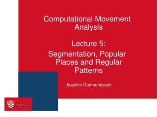
Computational Movement Analysis Lecture 1: Similarity Joachim Gudmundsson. Aim . Goal: Extract and make sense of information from trajectories (GPS, mobile, video, rfid …). Provide fundamental software tools to simplify and support qualitative analysis. Our model.

E N D
Computational Movement AnalysisLecture 1: SimilarityJoachim Gudmundsson
Aim Goal:Extract and make sense of information from trajectories (GPS, mobile, video, rfid…). Provide fundamental software tools to simplify and support qualitative analysis.
Our model Input: Locations sampled over time 30 0 31 5 28 6 38 12 25 53 48 47 16
Our model Input: Locations sampled over time Assumptions: a)Straight-line movement between consecutive samples b) Constant velocity 30 0 31 5 28 6 38 12 25 53 48 47 16
Brownian bridge movement model Input: Locations sampled over time Other models? Brownian bridge Brownian motion conditioned under starting and ending position Probability that object visits region A
Our model Input: a sequence of (x,y,t) - coordinates and a time stamp for example GPS data, mobile phone, radar, …
Additional information Input: a sequence of (x, y, t, z, temperature, speed, direction…)
Applications: Behavioural ecology • Migration patterns • “Popular places” • Home region • …
Applications: Behavioural ecology • Migration patterns • “Popular places” • Home range • Flock movements • …
Applications: Behavioural ecology • Interaction between jackdaws? • Effect of external factors ? [Joint work: Georgina Wilcox, Kevin buchin, MaikeBuchin, Ran Nathan and Anael Engel]
Applications: Behavioural ecology Behavioural ecology Short term: • Annual migration behaviour • Automatically detect activity • Home range Long term: - Foraging search strategies - Factors that may influence animal movement - How changes in the environment affects wildlife
Applications: Sport Data Accuracy: 100 mm Frequency: 25Hz [Joint work: Thomas Wolle and many others]
Applications: Sport • Tools to support sports analysts and coaches • Evaluate a players ability to pass (receive, execute…) • Evaluate a players ability to move into open areas • Evaluate a players ability to follow instructions • Detect frequent movement patterns • Detect correlations between players’ movement • Detect frequent passing patterns • Analyse turn-overs • Which events change the intensity of the game? • …
Applications: Hurricanes Goal: Early detection of hurricanes that may hit land
Applications: Transport • Collision prevention • Maximize unloading/loading
Applications: Shopping behaviour • Detect movement patterns • Change structure of shop to increase sales?
Examples of general problems • General problems • Repetitive patterns • Popular places • Trajectory segmentation • Trajectory simplification • Trajectory clustering • Subtrajectory clustering • Movement patterns • Single file • Formations • Leadership • Meetings • …
Seminar schedule • Lecture 1: Similarity • Lecture 2: Curve clustering • Lecture 3: Simplification • Lecture 4: Movement patterns • Lecture 5: Trajectory segmentation
Fundamental tools: clustering When are two trajectories similar? In most cases the spatial similarity is much more important than the temporal aspect.
Similarity of curves…measurements Agrawal, Lin, Sawhney & Shim, 1995 Alt & Godau, 1995 Yi, Jagadish & Faloutsos, 1998 Gaffney & Smyth, 1999 Kalpakis, Gada & Puttagunta, 2001 Vlachos, Gunopulos & Kollios, 2002 Gunopoulos, 2002 Mamoulis, Cao, Kollios, Hadjieleftheriou, Tao & Cheung, 2004 Chen, Ozsu & Oria, 2005 Nanni & Pedreschi, 2006 Van Kreveld & Luo, 2007 Gaffney, Robertson, Smyth, Camargo & Ghil, 2007 Lee, Han & Whang, 2007 Buchin, Buchin, van Kreveld & Luo, 2009 Agarwal, Aranov, van Kreveld, Löffler & Silveira, 2010 Sankaraman, Agarwal, Molhave, Pan and Boedihardjo, 2013 ...
Similarity measures Input: Two polygonal curves P and Q of size m in Rd Approach: Map curve into a point in dm-dimensional space 2D 10D
Similarity measures Input: Two polygonal curves P and Q of size m in Rd Approach: Map curve into a point in dm-dimensional space Similar? 10D 2D
Similarity measures Input: Two polygonal curves P and Q of size m in Rd Approach: Map curve into a point in dm-dimensional space Drawbacks: P and Q must have same number points Only takes the vertices into consideration Not similar 6D 2D
Similarity measures: Hausdorff Input: Two polygonal curves P and Q in Rd Distance:Hausdorff distance H(PQ) = maxpPminqQ |p-q| dH(P,Q) = max [H(PQ), H(QP)]
Similarity measures: Hausdorff Input: Two polygonal curves P and Q in Rd Distance:Hausdorff distance H(PQ) = maxpPminqQ |p-q| dH(P,Q) = max [H(PQ), H(QP)] P P Q Q
Similarity measures: Hausdorff Input: Two polygonal curves P and Q in Rd Distance:Hausdorff distance H(PQ) = maxpPminqQ |p-q| dH(P,Q) = max [H(PQ), H(QP)] P Q Drawbacks: Fail to capture the distance between curves.
Similarity measures: Fréchet Input: Two polygonal curves P and Q in Rd • Other interesting measures are: • Dynamic Time Warping (DTW) • Longest Common Subsequence (LCSS) • Model-Driven matching (MDM) • Drawback:Non-metrics (triangle inequality does not hold) which makes clustering complicated.
Similarity measure: Fréchet Distance Fréchet Distance measures the similarity of two curves. Dog walking example • Person is walking his dog (person on one curve and the dog on other) • Allowed to control their speeds but not allowed to go backwards! • Fréchet distance of the curves: minimal leash length necessary for both to walk the curves from beginning to end
Fréchet Distance Fréchet Distance measures the similarity of two curves. Dog walking example • Person is walking his dog (person on one curve and the dog on other) • Allowed to control their speeds but not allowed to go backwards! • Fréchet distance of the curves: minimal leash length necessary for both to walk the curves from beginning to end
Fréchet Distance Input: Two polygonal chains P=p1, … , pn and Q=q1, … , qm in Rd. The Fréchet distance between P and Q is: where and range over all continuous non-decreasing reparametrizations. Note that (0)=p1, (1)=pn, (0)=q1 and (1)=qm. Well-suited for the comparison of curves since it takes the continuity of the curves into account. (P,Q) =
Discrete Fréchet Distance The discrete Fréchet distance considers only positions of the leash where its endpoints are located at vertices of the two polygonal curves and never in the interior of an edge. May give large errors!
Compute the continuous Fréchet distance Input: Two polygonal chains P=p1, … , pnand Q=q1, … , qm in Rd. Decision problem:F(P, Q) ≤ r ? P P Q Q
Compute the Fréchet distance Input: Two polygonal chains P=p1, … , pnand Q=q1, … , qm in Rd. Decision problem:F(P, Q) ≤ r ? P P Q Q
Compute the Fréchet distance Input: Two polygonal chains P=p1, … , pnand Q=q1, … , qm in Rd. Decision problem:F(P, Q) ≤ r ? P P Q Q
Compute the Fréchet distance Input: Two polygonal chains P=p1, … , pnand Q=q1, … , qm in Rd. Decision problem:F(P, Q) ≤ r ? P P Q r Q
Compute the Fréchet distance Input: Two polygonal chains P=p1, … , pnand Q=q1, … , qm in Rd. Decision problem:F(P, Q) ≤ r ? P P Q Q
Compute the Fréchet distance Input: Two polygonal chains P=p1, … , pnand Q=q1, … , qm in Rd. Decision problem:F(P, Q) ≤ r ? P r P Q Q
Compute the Fréchet distance Input: Two polygonal chains P=p1, … , pnand Q=q1, … , qm in Rd. Decision problem:F(P, Q) ≤ r ? P r P Q Q
Compute the Fréchet distance Input: Two polygonal chains P=p1, … , pnand Q=q1, … , qm in Rd. Decision problem:F(P, Q) ≤ r ? P P Q Q
Compute the Fréchet distance Input: Two polygonal chains P=p1, … , pnand Q=q1, … , qm in Rd. Decision problem:F(P, Q) ≤ r ? P P Q Q
Compute the Fréchet distance Input: Two polygonal chains P=p1, … , pnand Q=q1, … , qm in Rd. Decision problem:F(P, Q) ≤ r ? P P Q Q
Compute the Fréchet distance Input: Two polygonal chains P=p1, … , pnand Q=q1, … , qm in Rd. Decision problem:F(P, Q) ≤ r ? P P Q Q
Compute the Fréchet distance Input: Two polygonal chains P=p1, … , pnand Q=q1, … , qm in Rd. Decision problem:F(P, Q) ≤ r ? P P Q Q
Compute the Fréchet distance Input: Two polygonal chains P=p1, … , pnand Q=q1, … , qm in Rd. Decision problem:F(P, Q) ≤ r ? P P Q Q
Compute the Fréchet distance Input: Two polygonal chains P=p1, … , pnand Q=q1, … , qm in Rd. Decision problem:F(P, Q) ≤ r ? P P Q Q
Compute the Fréchet distance Input: Two polygonal chains P=p1, … , pnand Q=q1, … , qm in Rd. Decision problem:F(P, Q) ≤ r ? P P Q Q
Compute the Fréchet distance Input: Two polygonal chains P=p1, … , pnand Q=q1, … , qm in Rd. Decision problem:F(P, Q) ≤ r ? P P Q Q
Compute the Fréchet distance Input: Two polygonal chains P=p1, … , pnand Q=q1, … , qm in Rd. Decision problem:F(P, Q) ≤ r ? Freespace diagram of P and Q free space P Q