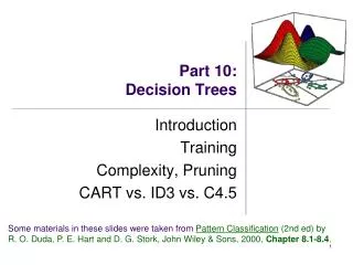
Part 10: Decision Trees

1. Part 10:Decision Trees Introduction Training Complexity, Pruning CART vs. ID3 vs. C4.5 Some materials in these slides were taken fromPattern Classification (2nd ed) by R. O. Duda, P. E. Hart and D. G. Stork, John Wiley & Sons, 2000, Chapter 8.1-8.4.

2. Introduction • Consider a classification problem where features are categorical or ordinal data • Cannot easily measure ‘distance’ between two feature vectors. • Instead of feature vectors, consider lists of attributes • e.g. represent fruit using 4-tuple {red, shiny, sweet, small} • Turn to non-metric methods such as decision trees, rule-based systems, grammars, etc. • Decision trees simple but effective method of pattern classification • Often reach same accuracy as ANN, K-NN • Clear interpretation of the resulting classifier • As opposed to ANN’s… • Can express as rules • e.g. if shape=thin AND colour=yellow  banana • Analogous to “20 questions” game.

3. Example Decision Tree or large?

4. Classification Based on DT • Classification of a sample from a decision tree (DT) is straightforward: • Start at the root node. • Apply the prescribed test on the feature contained in the root node. • Proceed down to the correct child • If it is a leaf node, apply class label for that node. Done. • Else, apply the prescribed test at that node. • Continue down tree in this manner until leaf reached. • One advantage: not all features must be measured to make a decision in some cases. • Big advantage when tests are costly (e.g. medical tests) • For numerical data, decision boundaries are parallel to feature axes (see next slide):

5. Decision Boundaries

6. Training DTs • How to train/build a DT from sample training data? • Once we have labelled training data, we have already decided on which features will be measured. • How to organize in a tree? • Adding tests (i.e. nodes) divides our training data into subsets. • Ideal if each subset had the same class ID • i.e. the node becomes “pure” • However, not typically the case. Therefore must either: • Decide to stop splitting and accept imperfect decision • Or, find another property to split on.

7. Training DTs: CART • CART (classification and regression trees) • DT training framework based on 6 questions: 1) Should the properties be restricted to binary-valued or allowed to be multi-valued? • How many decision outcomes or splits will there be at a node? (branching factor of the node limited to 2?) 2) Which property should be tested at a node? 3) When should a node be declared a leaf? 4) If the tree becomes ‘too large’, how can it be made smaller/simpler via pruning? 5) If a leaf node is impure, how should the category label be assigned? 6) How should missing data be handled?

8. Number of splits • Decision outcome at each node is called a split • Splits data into subsets • Branching factor/ratio is number of children from a node. • Can vary through tree, or be fixed. • Determining number of splits at a node is closely related to deciding which feature to split on • Any tree can be represented as a binary tree • See next slide

9. Binary tree structure

10. Query Selection & Node Impurity • Which feature to query at each node? • Want a simple, compact tree with few nodes (Occam’s razor) • Therefore each node should be chosen such that child subsets be as ‘pure’ as possible. • First, define impurity at node N: • Should be maximal for equal mix; reach zero for purely one class • a) Entropy impurity: • b) Variance impurity (2 class case): • Extend to multiple classes using Gini impurity • c) Misclassification impurity: • Min prob that training pattern misclassified at N Equal to prob of choosing wrong class randomly at node N

11. Measures of Node Impurity

12. Query Selection & Node Impurity • Examine features to look for greatest drop in impurity. • Reduction in impurity at node N: • (PL is fraction of patterns that go to NL) • If entropy measure is used, reduction in impurity is information gain (limited to 1 bit for binary splits) • Also search for optimal split point, s, for node T • e.g. once we choose to split on “weight”, must also define threshold value for split point (e.g. if w<1.5kg s=1.5) • Search simplified if you assume binary tree and tests are based on a single feature (monothetic tree).

13. Query Selection & Node Impurity • May find a range of optimal split points • Typically choose median/mean of range. • Greedy search – finds local optimum • Testing one node at a time, in isolation. • Gini vs. misclassfication impurity • Gini often preferred since it ‘anticipates future splits’. • e.g. have 90 w1 and 10 w2 at node N. Assume no split point leads to w2 majority in either child  misclassification impurity unchanged at 0.1. Gini would prefer a split that leads to L={70 w1, 0 w2} and R={20 w1, 10 w2} • In practice, pruning and stopping criteria have a bigger impact than impurity measure on final tree.

14. When to Stop Splitting • If we grow until each leaf contains a single sample, will have perfect purity  almost certainly overfit. • Several strategies: • 1) Make use of validation (hold-out) or n-fold cross-validation • Stop when minimum error reached on validation data • 2) Stop when ∆i gets too small • Apply at each node (not global stop)  leads to different depths in different branches. • Leads to an unbalanced tree • 3) Stop when node represents very few training samples • e.g. fewer than 5% of total training data • Benefits analogous to k-NN (density of data defines decision partition size)

15. When to Stop Splitting • Several strategies: • 4) Minimize tree complexity and total node impurity: • Related to MDL if entropy used for i(N): Total i(N) of all leaves measure uncertainty of data, given model represented by tree; size of tree is measure of model complexity. • 5) Test of significance • a) Form population of ∆i(N) from tree. Only accept a new split if new ∆i is significantly different from zero (X2test) • b) Form null hypothesis that split is equivalent to random. Test if observed distribution of class labels is significantly different. degrees of freedom = 1 nie=Pni, niL= # wi sent left by proposed split

16. Pruning • Can stop prematurely from lack of sufficient ‘look ahead’ – horizon effect • When determining whether to stop splitting, we don’t consider quality of splits at child nodes • Biases learning algorithm to trees with greatest impurity reduction is near the root node • Alternative is pruning • Grow tree completely, then eliminate/prune/merge pairs of leaf nodes when gain in impurity < T • For large datasets, computational complexity of pruning may be too high. Otherwise, use it! • Can prune non-leaf nodes, replacing subtree with a leaf, or removing decision node and replacing with a child node.

17. Example 1: Stability of DT Training • Small changes in the training data can lead to large differences in final classification boundaries • Example: Consider 16 training points with 2 features. Build a binary CART tree using entropy: x2 value could be .36 or .32

18. Example 1 – Unpruned Trees Tree 1: Assume x2 was .36 impurity shown in courier impurity of leaf nodes = 0 Tree 2: Assume x2 was .32

19. Example 1: Sample Calculations • Small change in one measured feature results in vastly different classification boundaries. • Sample calculations: • Impurity at root node is: • Split point of test @ root: • Try all n-1=15 possible split points in each dimension • Greatest reduction in impurity occurs near x1s=0.6 • If pruning were applied, shaded subtree (pair of leaf nodes) would be first deleted/merged/pruned • Would lead to smallest gain in impurity

20. Feature Selection, Multivariate DTs, & Unbalanced training sets • Tree learning will not work well if individual features do not discriminate data well • See next slide • Can preprocess data • E.g. run PCA first, then build tree on principal components. • Otherwise can permit more complicated decisions at nodes, involving multiple features • See next, next slide. • Unbalanced training set • Can use loss function to weight errors in under-represented class more heavily • Weighted Gini impurity:

23. Missing Attributes • May have missing attributes: • i) During training • Instead of throwing out deficient patterns, instead calculate impurity at each node using only attribute information that is present. • Calculate best split point using data available • ii) During classification • Use primary decision at a node whenever possible, use alternative tests when not available. • During training, in addition to identifying optimal split at each node, also provide surrogate splits(label & rule) • Maximize ‘predictive association’ with primary split • e.g. look for similar splits between left/right children • Analogous to replacing missing value by nonmissing attribute most correlated with it. The fact that an attribute is missing, may be informative and may become a separate test.

24. Example 2: Surrogate Splits f1 f2 f3 3 features for each sample f1, f2, f3 f1 f3 f2 Minimizes entropy Mimics primary split using different attribute Likewise, but not as well…

25. Other DT Packages • ID3 • Uses only nominal (unordered data) • Real-valued data are binned first (discards ordering information). • Branching factor is always equal to number of nominal values/bins for that variable • Use ‘ratio impurity’ which penalizes for number of splits • Tree depth is always equal to number of features • Algorithm continues until all nodes are pure • C4.5 • Successor to ID3 • Real-valued data treated like CART • Branching factor same as ID3 for nominal data • Pruning using statistical significance of splits. • In case of missing data during classification, follow all possible branches, then use weighted voting on final leaf nodes.