Download
1 / 15
150 likes | 388 Vues
Secondary upwelling instabilities developed in high Rayleigh number convection. Fabien Dubuffet 1 , M.S. Murphy 2 , Ludek Vecsey 3 , Erik O. Sevre 1 and David A. Yuen 1.

E N D
Secondary upwelling instabilities developed in high Rayleigh number convection Fabien Dubuffet1, M.S. Murphy2, Ludek Vecsey3, Erik O. Sevre1 and David A. Yuen1 1 Department of Geology and Geophysics and Minnesota Supercomputing Institute, University of Minnesota, Minneapolis, MN 55415-0227, USA. 2 Department of Geology, Colby College, Waterville, ME 04901, USA. 3 Department of Geophysics, Charles University, 1800 Prague 8, Czech Republic.
Whitehead's Laboratory Experiments The behavior observed by Skillbeck and Whitehead (1978) when a fluid of lower density and lower viscosity was injected into a fluid of higher density and higher viscosity at an angle of 25 degrees and allowed to propogate for two minutes.Figure courtesy of Jack Whitehead
Apparatus constructed by Whitehead in 1982 to conduct his second series of experiments with tilted conduits. The rotating apparatus in the upper portion of the tank creates a zone of shear that bends the conduit as it flows upward. Resulting shadowgraph of instabilities forming from a conduit
The numerical models • Boussinesq approximation. • Infinite Prandtl Number • 2-D model: • - two-dimensional axisymmetric model in a spherical shell (core radius 0.55). • fourth-order finite-difference method to solve for the vorticity, stream function, and the temperature field. • up to 3400 x 500 grid points. • 3-D model: • Cartesian geometry ( aspect ratio 3). • Stokes equation : Fast Fourier transform along the horizontal axis and finite differences. • Temperature equation : A.D.I. • up to 385 x 385 x 385 grid points.
Ra = 3x10⁶ Ra = 3x10⁷
Ra = 3x10⁸ Ra = 109
Ra = 3x10⁹ time
Ra = 5x10⁹ Ra = 1010
Wavelength Argument - There is no unique wavelength but a broadband spectrum of possible folding wavelengths. - The variations of the bandwidth will be used to constrain the possible range of secondary folding instabilities
Major islands of the state of Hawaii Figure modified from Cox (1999)