Download
1 / 30
520 likes | 1.93k Vues
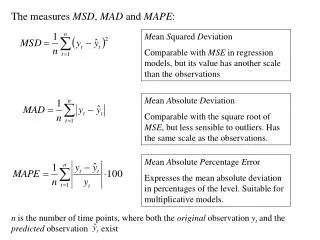
The measures MSD , MAD and MAPE :. M ean S quared D eviation Comparable with MSE in regression models, but its value has another scale than the observations. M ean A bsolute D eviation

E N D
The measures MSD, MAD and MAPE: Mean Squared Deviation Comparable with MSE in regression models, but its value has another scale than the observations Mean Absolute Deviation Comparable with the square root of MSE, but less sensible to outliers. Has the same scale as the observations. Mean Absolute Percentage Error Expresses the mean absolute deviation in percentages of the level. Suitable for multiplicative models. n is the number of time points, where both the original observation ytand the predicted observation exist
Modern methods • The classical approach:
Explanation to the static behaviour: The classical approach assumes all components except the irregular ones (i.e. tand IRt ) to be deterministic, i.e. fixed functions or constants To overcome this problem, all components should be allowed to be stochastic, i.e. be random variates. A time series yt should from a statistical point of view be treated as a stochastic process. We will interchangeably use the terms time series and process depending on the situation.
Stationary and non-stationary time series • Characteristics for a stationary time series: • Constant mean • Constant variance • A time series with trend is non-stationary!
Box-Jenkins models A stationary times series can be modelled on basis of the serial correlations in it. A non-stationary time series can be transformed into a stationary time series, modelled and back-transformed to original scale (e.g. for purposes of forecasting) ARIMA– models Auto Regressive, Integrated, Moving Average This part has to do with the transformation These parts can be modelled on a stationary series
Different types of transformation 1. From a series with linear trend to a series with no trend: First-order differences zt = yt – yt – 1 MTB > diff c1 c2
2. From a series with quadratic trend to a series with no trend: Second-order differences wt = zt – zt – 1 = (yt – yt – 1) – (yt – 1 – yt – 2) = yt – 2yt – 1 + yt – 2 MTB > diff 2 c3 c4
3. From a series with non-constant variance (heteroscedastic) to a series with constant variance (homoscedastic): Box-Cox transformations (per def 1964) Practically is chosen so that yt + is always > 0 Simpler form: If we know that yt is always > 0 (as is the usual case for measurements)
The log transform (ln yt) usually also makes the data ”more” normally distributed Example: Application of root (yt) and log (ln yt ) transforms
AR-models (for stationary time series) Consider the model yt = δ + ·yt –1 + at with {at }i.i.d with zero mean and constant variance = σ2 and where δ (delta) and (phi) are (unknown) parameters Set δ = 0by sake of simplicity E(yt) = 0 Let R(k) = Cov(yt,yt-k) = Cov(yt,yt+k) = E(yt ·yt-k) = E(yt ·yt+k) R(0) = Var(yt) assumed to be constant
Now: • R(0) = E(yt ·yt) = E(yt ·(·yt-1 + at) = · E(yt ·yt-1) + E(yt ·at) = • = ·R(1) + E((·yt-1 + at)·at) = ·R(1) + · E(yt-1·at) + E(at ·at)= • = ·R(1) + 0 + σ2 (for atis independent of yt-1) • R(1) = E(yt ·yt+1) = E(yt ·(·yt + at+1) = · E(yt ·yt) + E(yt ·at+1) = • = ·R(0) + 0 (for at+1is independent of yt) • R(2) = E(yt ·yt+2) = E(yt ·(·yt+1 + at+2) = · E(yt ·yt+1) + • + E(yt ·at+2) = ·R(1) + 0 (for at+1is independent of yt) •
R(0) = ·R(1) + σ2 • R(1) = ·R(0) Yule-Walker equations • R(2) = ·R(1) • … • R(k ) = ·R(k – 1) =…= k·R(0) • R(0) = 2 ·R(0)+ σ2
Note that for R(0) to become positive and finite (which we require from a variance) the following must hold: This in effect the condition for an AR(1)-process to be weakly stationary Note now that
ρkis called the Autocorrelation function (ACF) of yt ”Auto” because it gives correlations within the same time series. For pairs of different time series one can define the Cross correlation function which gives correlations at different lags between series. By studying the ACF it might be possible to identify the approximate magnitude of
The look of an ACF can be similar for different kinds of time series, e.g. the ACF for an AR(1) with = 0.3 could be approximately the same as the ACF for an Auto-regressive time series of higher order than 1 (we will discuss higher order AR-models later) To do a less ambiguous identification we need another statistic: The Partial Autocorrelation function (PACF): υk = Corr (yt ,yt-k | yt-k+1, yt-k+2 ,…, yt-1 ) i.e. the conditional correlation between yt and yt-kgiven all observations in-between. Note that –1 υk 1
A concept sometimes hard to interpret, but it can be shown that for AR(1)-models with positive the look of the PACF is and for AR(1)-models with negative the look of the PACF is
Assume now that we have a sample y1, y2,…, ynfrom a time series assumed to follow an AR(1)-model. Example:
The ACF and the PACF can be estimated from data by their sample counterparts: • Sample Autocorrelation function (SAC): • if n large, otherwise a scaling • might be needed • Sample Partial Autocorrelation function (SPAC) • Complicated structure, so not shown here
The variance function of these two estimators can also be estimated Opportunity to test H0: k= 0 vs. Ha: k 0 or H0: k= 0 vs. Ha: k 0 for a particular value of k. Estimated sample functions are usually plotted together with critical limits based on estimated variances.
Example (cont) DKK/USD exchange: SAC: SPAC: Critical limits
Ignoring all bars within the red limits, we would identify the series as being an AR(1) with positive . The value of is approximately 0.9 (ordinate of first bar in SAC plot and in SPAC plot)
Higher-order AR-models AR(2): or yt-2 must be present AR(3): or other combinations with 3 yt-3 AR(p): i.e. different combinations with p yt-p
Stationarity conditions: For p > 2, difficult to express on closed form. For p = 2: The values of 1 and 2 must lie within the blue triangle in the figure below:
Typical patterns of ACF and PACF functions for higher order stationary AR-models (AR( p )): ACF: Similar pattern as for AR(1), i.e. (exponentially) decreasing bars, (most often) positive for 1positive and alternating for 1 negative. PACF: The first p values of k are non-zero with decreasing magnitude. The rest are all zero (cut-off point at p ) (Most often) all positive if 1 positive and alternating if 1 negative
Examples: AR(2), 1positive: AR(5), 1 negative: