Download
1 / 38
390 likes | 563 Vues
Open Economy. Presence of foreign sector Trade Investment. Trade. Y = C + I + G + X – M M – imports Consumer spending on foreign output Investment spending on foreign output Government spending on foreign output X – exports Foreign spending on domestic output.

E N D
Open Economy • Presence of foreign sector • Trade • Investment
Trade Y = C + I + G + X – M • M – imports • Consumer spending on foreign output • Investment spending on foreign output • Government spending on foreign output • X – exports • Foreign spending on domestic output
Spending and Output in an open economy • At any given time period a country’s spending need not equal its output • NX<0 a country spends more than it produces, i.e. borrowing • NX>0 a country’s production exceeds its spending, i.e. lending
National Savings in Open Economy • NS = Y – C – G = I + NX • NX = NS – I • NX>0 accumulation of foreign financial assets • NX<0 sale of domestic financial assets to foreigners • Trade balance = net capital flow • US BoP (www.bea.gov) • Current Account – Trade • Financial Account – Investment
Small Open Economy • Incapable of causing changes in the world’s financial markets, i.e. is a price taker in financial markets, unable to influence the price of loanable funds in the global markets – interest rate. S (domestic+foreign) r I Fiscal Policy in a small open economy Monetary Policy in a small open economy
example • Consider a closed economy with • Y=20000 • G=T=0 • C=1000+0.8*(Y-T) • I=5000-500 r ----------------------------------------------------------- • What is the level of interest rate? ----------------------------------------------------------- Now, assume this is a small open economy and the global interest rate is 5% • Would this country be a net borrower or lender? • What would the level of net exports be? • Now, assume that the level of government spending increases to 3000, would this country be a net borrower or lender? And what would the level of NX be? • Now assume that G is reduced to 0, but T is reduced to -1000, what would be the level of NX? • Now assume that G=T=0, but the investment function changes to: I=8000-500r
Exchange Rate • Translating Factor • Nominal Exchange Rate • Simple conversion • Demand for the currency • Exports • Foreign investment into domestic economy • Central banks expanding their holdings of domestic currency • Supply of the currency • Imports • Domestic investment overseas • Central banks selling holdings of the domestic currency • Purchasing Price Parity • Real Exchange Rate • NX and the terms of trade
Real exchange rate • Real Exchange rate • Terms of exchange (“terms of trade”) • Relative price • RE = NE * Pd/Pf • Overvalued versus undervalued currency and the real exchange rate • Net Exports and the real exchange rate • Fiscal expansion • Decline in National Savings Increase in influx of foreign investment appreciation of the currency deterioration of trade balance • Monetary expansion • Increase in domestic money supply inflation deterioration of trade balance influx of foreign investment • Trade restrictions • Net exports function increases the real exchange rate appreciates by the impact of the trade restriction on the relative price
Purchasing Price Parity • “same things should cost the same price world over” • Price of oil • Real exchange rate = 1 • REd = NEd * Pd/Pf = 1 NEd = Pf/Pd (absolute PPP) • Nominal exchange rate is driven by the difference in the rates of inflation • %change in NE = inflation f – inflation d [relative PPP] • If (inflation f > inflation d) then DC appreciates • If (inflation f < inflation d) then DC depreciates • Tradable versus non-tradable internationally goods • Consumer preferences
Business Cycle • Short-run versus Long-run macroeconomics • Sticky Prices • Contractual arraignments and wages • 2001-present airfares and the price of oil • Output/Employment adjustments and the profit equation
Output/Employment/Inflation and the business cycle • Recession • Expansion • Natural Unemployment • Relationship between unemployment and inflation
Indicators of future/current change in the business cycle • Leading Indicators • Business inventories • Average Work hours in manufacturing • Average weekly claims for unemployment insurance • New orders for non-defense capital goods • Sales tax receipts • Construction employment • Residential permits • Stock index (index futures) • Growth in wage rate • Interest rate spread (e.g. 10 year versus 1 year bond)
More on indicators • Coincident indicators • Total hours worked • Value of unemployment claims • Total tax revenues • Corporate income tax receipts
The simple Keynesian Theory of Income Determination • Planned versus unplanned expenditures • Planned • “long-run” equilibrium • A situation where all sectors (households, firms, government, foreigners) want to spend exactly the amount of income that is being generated by the current level of production • C, Ip, G, NX Ep = C + Ip + NX • Unplanned • “Short-run” equilibrium • Iu = change in business inventories (unintended inventory investment) • Autonomous versus induced expenditures • Consumption function
The Keynesian Cross Actual Expenditures Planned expend Planned Expenditures equilibrium Ap Real Income (Y) Note: MPC is the slope of the Ep function
Investment and Savings E(r2) E • I = I (r) Planned investment is a function of real interest r1>r2 E(r1) Y r r1 r2 Y
The mechanics of the IS curve • Functional form of the IS curve • Y = f (r, other factors) • Movement along the curve • Changes in the interest rate • Shifts of the IS curve • Anything (other than the interest rate) that changes the autonomous planned expenditures • Rotation of the curve • Changes in the multiplier • The greater is the multiplier, the flatter is the IS curve (more sensitive to the interest rate changes) • Sensitivity of the Investment component to changes in the interest rate
Simple review questions • What should happen to the IS curve in each of the following cases? • Government spending increases • Autonomous taxes increase • mpc increases • mps decreases • Income tax rate increases • Autonomous consumption increases
Money Market (review) • Equilibrium in the money market • Real Money Demand: Md/P = f (r, Y, P) • Interest rate!!! Recall the opportunity cost of money • Y!!! Recall the transactional demand for money • Real Money Supply: Ms/P = f (Policy, Price level) • NOT a function of the interest rate r Ms/P Md/P Real money balance
Liquidity and Money • Combinations of Y and r for which the money market is in equilibrium r r Ms/P LM L(Y2) L(Y1) Y2>Y1 RMB Y1 Y2 Y
Dynamics of the LM curve • Shifts in the LM • Money Supply changes • Changes in the Price Level (P) • Rotation • Anything that makes the demand for money less sensitive to the interest rate makes both, the money demand and the LM curve steeper (rotating it upward around the horizontal intercept)
Monetary Policy • Strong Monetary Policy • Flat IS curve • Strong dependency of investment and consumption on the interest rate • Steep LM curve • Weak responsiveness of the demand for money to interest rate changes; thus, large changes in the interest rate are needed to readjust the money market. The larger is the change in the interest the stronger is the stimulus to I and C, and hence the effect on the IS curve, and the GDP. • Weak Monetary Policy • Steep IS Curve • Weak dependency of I and C on the interest rate • Flat LM curve • High responsiveness of the demand for money to interest rate changes • small changes in the interest rate have large impact on the asset allocation of the household (between money (M1) and less liquid, interest earning assets) • Horizontal LM curve and the Liquidity Trap
Fiscal Policy • Strong Fiscal Policy • Flat LM curve • Strong sensitivity of the demand for money to interest rate changes, hence no large interest rate changes needed to readjust the money market, hence limited crowding out effect • Steep IS curve • Low sensitivity of I and C to interest rate changes, hence limited crowding out effect • Weak Fiscal Policy • Flat IS curve • Strong crowding out effect • Steep LM curve • Low sensitivity of money demand to interest rate changes requires large change in the interest rate to readjust the money market to
Aggregate Demand – Aggregate Supply and Inflation • Aggregate Demand • Shows different combinations of the price level and real output at which the money and commodity markets are both in equilibrium • Summarizes the effects of changing prices on the level of real income. • Is derived from the IS-LM equilibrium • Recall: IS represents equilibrium in the commodity market and LM represents equilibrium in the money market
Deriving AD r LM1(P1) LM2(P2) As P decreases the real Money supply increases, thus the LM curve shifts outwards, leading to a higher equilibrium level of Y IS Y P P1 P2 AD Y
AD curve continued • Shifts of the AD curve • Shifts in the IS curve • Shifts in the LM curve • Slope of the AD • Slope of the IS (multiplier) • Slope of the LM curve
Aggregate Supply • Long-Run • Capacity based, full price flexibility • Short-Run • Horizontal: all prices fixed • Upward slopped: sticky-wages model • Input costs are assumed to be fixed • If output prices change real input prices change, causing changes in firms behavior
Policy in Open Economy • Assumptions • Small economy • No capital mobility restrictions • Conclusion • Interest rate is fixed to the world interest rate
Monetary Policy • Floating exchange rate regime: • Monetary expansion leads to currency depreciation • Fixed exchange rate regime: • Monetary policy is ineffective (EU12)
Fiscal Policy • Floating exchange rate regime • Currency appreciation makes fiscal expansion ineffective • Fixed exchange rate regime • Fiscal expansion leads to monetary expansion
The Economic Development • Output per capita • Sources of growth: • resources • Land • Capital • Human capital • Technological progress • Institutional development
The Solow Growth Model – Part Isupply side • Y = F (K,L) • To convert to per-worker output measure we must assume CRTS: • zY = F (zK, zL) • Per Capita (per worker) output measure: • y = f (k) • Assume diminishing MPK property
The Solow Growth Model – Part Idemand side • Output is allocated between consumption and investment (savings translate into investment) • y = c + i; i = sY, where s represents the savings rate • Consumption of fixed capital, i.e. depreciation dk • Capital evolution (formation) equation:
The Solow Growth Model – Part Idemand side • Output is allocated between consumption and investment (savings translate into investment) • y = c + i; i = sY, where s represents the savings rate • Consumption of fixed capital, i.e. depreciation dk • Capital evolution (formation) equation: Dk = i - dk
The Solow Growth Model – Part Isteady state • Capital stock remains the same over time • Dk = 0 sf(k) = dk • Convergence to the steady state • The Golden Rule of Capital Stock • Maximization of consumption • c = y – i in Steady State i = dk • c = f(k) – dk • MPk = d