Download
1 / 11
110 likes | 245 Vues
Roughing-out of statistical data. Calculation of numerical descriptions. Today we will talk about the roughing-out of statistical data. It is such type of treatment, which is used with the purpose of receipt of initial picture about the results of experiment.

E N D
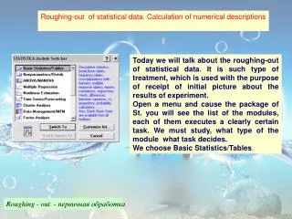
Roughing-out of statistical data. Calculation of numerical descriptions Today we will talk about the roughing-out of statistical data. It is such type of treatment, which is used with the purpose of receipt of initial picture about the results of experiment. Open a menu and cause the package of St. you will see the list of the modules, each of them executes a clearly certain task. We must study, what type of the module what task decides. We choose Basic Statistics/Tables. Roughing-out - первичная обработка
A window will appear with an empty table measuring 10 lines and 10 columns. The list of the submodules is visible in a window Описательные статистики Корреляционные матрицы t- критерий для оценки средних значений в двух группах; t- критерий для оценки значимости различий двух групп; Однофакторный дисперсионный анализ; Вариационные таблицы; Табличное представление информации; Калькулятор вероятностных распределений; Другие критерии значимости.
We will consider a task for an example. In Excel data are entered about estimations which got students of two groups on examination. It is necessary to compare results, in what group students have higher estimations. An estimation is a variable quantity. At first it is needed to define the type of this variable. It variable is named random. A random value is a value, accepting as a result of experiment that or another value depending on the random end of test. They are divided by 2 classes: discrete and continuous. A discretevalue accepts eventual or endless, but the countable set of values is obligatory, it values can be disposed in the certain order and number. For example, an amount of students in a group, going in for exam, is a discrete value. An amount of days of work of device is a - random value. An amount of points, falling out on boneis a discrete random value. Continuous - it values fill some area of space, volume or time, it is an abscissa of point of hit at a shot, time of faultless work of device, size of wear of detail. eventual – конечный, возможный obligatory - обязательный
Copy basic data in Statistica. I remind, the amount of columns is equal two, the amount of lines is equal 25. You must increase the number of lines on 15 and decrease the amount of columns on seven. A table, consisting of three columns and 25 lines, must turn out for you. Give the name to the columns by means of the button Group 1 and Group 2
The roughing-out of discrete values consists of next actions: • To find frequency of appearance of it values. For example, in our table in the first group such estimations were got: • 2- 5 • 3-4 • 4-13 • 5- 3 • It is frequencies of reiterations. They are designated by mx Then determine frequentness on a formula wx= mx/N N is a total amount of data. Let us count up. Two it was got five. The common amount of data of N is equal to 25. Then mx =5/25=20%. Three it is got four, mx =4/25=16% Count up frequency for other estimations and enter it, using a pointer. For the call of pointer click into a sliding seat the right mouse button and choose a word Pointer (Erfpfntkm). Then choose his original appearance (Pen (Ручка) or marker (Фломастер)). You can choose a color (A color blackened – Цвет чернил). Write necessary numbers on the screen.
To turn off a pointer, once again right-click mouse on a screen and choose Pointer / of Shooter. To save the handwritten notes? (Сохранить рукописные примечания?) Press the button to Save (Сохранить). After it we will be able to check up the rightness of your calculations.
The next stage is calculations of the accumulated frequentness and frequency . Accumulated frequency and frequentness show shown frequentness with values by equal or less to given. For example,2 is got 5 times in the first group. The accumulated frequency is equal to 5, because there are not estimations, less 2. 3 it is got 4 times (it is frequency), if to lay down the amount of 3 and 2, will get 9. It is the accumulated frequency for an estimation 3. mxH - denotation of the accumulated frequency; wxH - is denotation of the accumulated frequentness; You will fill two last lines of table.
Now we must get the results of treatment обработкаin the package of STATISTICA. Open a menu of Analysis choose Frequency Table . A window will be Opened with the image of variants of roughing-out of data. It is needed to set one or a few variables are for treatment. For this purpose press on the button Variable. Now in a window on the right of the button the word of None is written - not a single variable is chosen for treatment.
Now we must get the results of treatment обработкаin the package of STATISTICA. Open a menu of Analysis choose Frequency Table . A window will be Opened with the image of variants of roughing-out of data. It is needed to set one or a few variables are for treatment. For this purpose press on the button Variable. All district values –for discrete values , all variable values are examined. No of Exact interval –used for treatment of continuous variables, it is here necessary to set, what number of intervals all range is broken up on, thus enter the number of intervals.
Neat–breaks up on the indicated number of intervals, here borders become round either to whole or a 1 sign after a comma. Step Size–size of interval. It is possible to set the size. Starting at –initial value of variable. Integer categories –we break up on the integer values of intervals. User –specified categories –to set dividing by groups on the principle include – включить, exclude – исключить.