Download
1 / 37
390 likes | 585 Vues
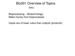
Bio301 Overview of Topics. Intro. Bioprocessing – Biotechnology: Make money from bioprocesses Inputs are of lower value than outputs (products) Computer based learning activities (CBLA) are on http://sphinx.murdoch.edu.au/units/extern/BIO301/teach/index.htm. Lecture overview L1-3.

E N D
Bio301 Overview of Topics Intro Bioprocessing – Biotechnology: Make money from bioprocesses Inputs are of lower value than outputs (products) Computer based learning activities (CBLA) are on http://sphinx.murdoch.edu.au/units/extern/BIO301/teach/index.htm
Lecture overview L1-3 Lecture 1: Intro, study guide, what is a bioreactor, Learning by interacting Lecture 2: What is diffusion, how can we predict the behaviour of a randomly moving molecule? moving dots, entropy, driving force, equilibrium, rate of diffusion, first order kinetics, kLa Lecture 3: oxygen transfer rate, kLa value. Graphical method of determining the kLa. Mathematical (2 point) determination of kLA Calculation and prediction of oxygen transfer as function of DO. Oxygen transfer efficiency. Bacterial OUR, DO. steady state
Molecular diffusion relies on random movement resulting in uniform distribution of molecules
Oxygen Transfer Rate (OTR) Overview Diffusion, how does it work, how can we predict it? Diffusion is random …. and yet predictable. A simple model simulation can show that although the diffusion movement is random, it can be precisely predicted for large number of molecules (e.g. Fick’s law of diffusion)
• • • • • • • • • • Oxygen Transfer Rate (OTR) (diffusion, convection) Low OTR High OTR Transfer by diffusion is extremely slow and depends on surface area Wind Oxygen transfer by convection (turbulences) is more efficient Air In • Bioreactors combine maximum convection with maximum diffusion • Course bubbles cause more convection, fine bubbles more diffusion How soluble is oxygen?
Oxygen solubility (cS) • The net transfer of oxygen from • gas phase to solution reaches a dynamic equilibrium • O2 input = O2 output • equilibrium results in defined saturation concentration (cs). • The saturation concentration is also the oxygen solubility • How soluble is oxygen?
Oxygen solubility (cS) Oxygen is not very polar poorly soluble in water. Oxygen Solubility is described by Henry’s Law which applies to all gases p = partial pressure of oxygen k = constant depending on gas type, solution and temperature cS = concentration of oxygen dissolved in water p = k*cS • Meaning: The amount of oxygen which dissolves in water is proportional to the amount of oxygen molecules present per volume of the gas phase. • Partial pressure ~ number of O2 molecules per volume of gas • increases with O2 concentration in gas • increases with total gas pressure • How to calculate partial pressure? (refer to CBLA)
Oxygen solubility (cS) Examples of using the proportionality between partial pressure of oxygen in the atmosphere and the saturation concentration cS: p = partial pressure of oxygen k = constant depending on gas type, solution and temperature cS = concentration of oxygen dissolved in water p = k*cS • If the reactor is operated under 2 times atmospheric pressure (200kPa instead of 100 kPa air pressure), the new saturation concentration will be abou 16 mg/L instead of 8 mg/L. • If air (partial pressure = 0.21* 100 kPa) is replaced by pure oxygen atmosphere (partial pressure 100kPa) the oxygen saturation concentration is about 40 mg/L (more precise 8*100/21) instead of 8 mg/L. • How to calculate partial pressure? (refer to CBLA)
468 cs = (31.6 + T) Oxygen solubility (cS) Effect of temperature Oxygen Saturation Concentration cs (mg/L) Temperature (°C) Oxygen solubility decreases with increasing temperature. Overall: oxygen is poorly soluble (8mg/: at room temp.) More important than solubility is oxygen supply rate (oxygen transfer rate OTR).
Oxygen Transfer Rate (OTR) (gradient, driving force) Question: What is the driving force for oxygen dissolution? At oxygen saturation concentration (cs): dynamic equilibrium exists between oxygen transferred from the air to water and vice versa. No driving force OTR Answer: The difference between cS and the actual dissolved oxygen concentration (cL) is the driving force. OTR is proportional to the that difference. Thus: OTR ~ (cS – cL) Need to determine the proportionality factor
8 Air On cL (ppm) 0 5 10 Time (min) OTR – depends on DO (cL) Significance of OTR: critical to know and to control for all aerobic bioreactors 1. Deoxygenation (N2, sulfite + Co catalyst) 2. Aeration and monitoring dissolved oxygen concentration (D.O. or cL) as function of time 3. OTR = slope of the aeration curve (mg/L.h or ppm/h)
OTR – depends on DO (cL) 4. Observation: OTR decreases over time (and with incr. cL) 5. OTR is not a good measure of aeration capacity of a bioreactor 6. OTR is highest at cL = zero (Standard OTR) 7. OTR is zero at oxygen saturation concentrations (cs) 8. OTR is negatively correlated to cL 9. OTR is correlated to the saturation deficit (cs - cL), which is the driving force for oxygen transfer 9. The factor of correlation is the volumetric mass transfer coefficient kLa OTR = kLa (cs - cL) Mg/L/h h-1 mg/L
OTR –Significance of gradient First: steep step in oxygen (top layer saturated, next layer oxygen free) Then: buildup of a gradient of many layers. Each layer is only slightly different from the next Transfer from layer to layer has little driving force. Gradient build-up inhibits fast diffusion
10. OTR is not a useful parameter for the assessment of the aeration capacity of a bioreactor. This is because it is dependent on the oxygen concentration (cL) 11. The kLa value is a suitable parameter as it divides OTR by saturation deficit: OTR (cs - cL) kLa = 12. kLa = the key parameter oxygen transfer capacity. How to determine it?
Lec 2 summary: • Oxygen is poorly soluble depending mainly on • partial pressure in headspace • Temperature • OTR is driven and proportional to driving force (cS-cL) • kLa is the proportionality factor (first order kinetics) • kLa describes the performance of a bioreactor to provide • Oxygen to microbes • Next lecture: quantify kLA
Lec 3 outlook: • Aeration curve • Quantify OTR at a given point of an aeration curve • Quick estimate of kLa • Graphical determination of kLa • Mathematical determination of kLa • Run computer simulation to obtain data • Oxygen transfer efficiency (OTE) • OTR proportional to cs-cL • OTR inverse proportional to cL
8 Air On 6 cL (mg/L) 5 mg/L 4.5 min 0 5 10 Time (min) OTR – Quick estimate of kLA Example: determine OTR at 6 mg/L OTR is the slope of the tangent for each oxygen concentration OTR = ∆ cL/ ∆ t = 5 mg/L/ 4.5 min = 1.1 mg/L/min = 66 mg/L/h
OTR – quick estimate of kLA kLa = OTR (cs-cL) = 66 ppm / h (8 ppm – 6 ppm) = 3.3 h-1 Q: Problem with this method? A: based on one single OTR slope measurement and unreliable to obtain from real data. DO Time
8 6 4 2 0 5 10 OTR – Graphical determination of kLa 1. Monitor aeration curve 2. Determine graphically the OTR at various oxygen concentrations (cL) At 6 ppm: OTR = 25 mg/L/h At 4 ppm: OTR = 50 mg/L/h cL (ppm) At 3 ppm: OTR = 60 mg/L/h At 0.5 ppm: OTR = 30 ppm/h Time (min) 3. Tabulate OTR and corresponding cL values cL (mg/L) Cs - cL (mg/L) OTR (mg/L/h) 0.5 3.0 4.0 6.0 8.0 7.5 5.0 4.0 2.0 0.0 30 60 50 25 0
70 mg/L/h kLa = = 12 h-1 6 mg/L OTR – Graphical determination of kLa 4. Plot OTR values as a function of cs - cL. Standard OTR 100 OTR (mg/L/h) cs 50 0 0 2 4 6 8 cs- cL (mg/L) 5. A linear correlation exists between kLa and the saturation deficit (cs - cL) which is the driving force of the reaction. 6. The slope of the plot OTR versus cs - cL is the kLa value. 7. The standard OTR (max OTR) can be read from the intercept with the cs line. (Standard OTR = 100 ppm/h)
2. kLa = dcL/dt (cs- cL) cs - co ( ) cs 3. kLa = ln cs - ci • ci = 6 ti - to Dissolved Oxygen Concentration (mg/L) • co = 3 to ti Time (min) = ln 2.5 8- 3 ppm ( ) kLa = ln 4.4 min 8 - 6 ppm 10.5 - 6.1 min Mathematical Determination of kLa 1. OTR is a change of cL over time, thus = dcL/dt Integration gives = 12.5 h-1 = 0.21 min-1
4. This method should be carried out for 3 to 4 different intervals. By aver 5. Once the kLa is known it allows to calculate the OTR at any given oxygen concentration: OTR = kLa (cs - cL)
Factors Affecting the Oxygen Transfer Coefficient kLa kLa consists of: • kL = resistance or thickness of boundary film • a = surface area Bulk Liquid Bubble [Oxygen] Cell Distance Main boundary layer = steepest gradient → rate controlling, driving force
Effect of Fluid Composition on OTR The transfer across this boundary layer increases with: • ↓ thickness of the film, thus ↑ degree of shearing (turbulence) • ↑ surface area • ↓ surface tension • ↓ viscosity (best in pure water) • ↓ salinity • ↓ concentration of chemicals or particles • detergents? • ↑ emulsifiers, oils, “oxygen vectors”
oxygen transferred OTE = oxygen supplied oxygen transferred (mol/L.h) X 100 % OTE = oxygen supplied (mol/L.h) Oxygen Transfer Efficiency (OTE) Significance of OTE: economical, evaporation Calculation of OTE (%): Why do students find this type calculation difficult? Units are disregarded. Molecular weights are misused.
3.1 (mmol/L.h) X 100 % OTE = 34.3 (mol/L.h) Oxygen Transfer Efficiency (OTE) A bioreactor ( 3 m3) is aerated with 200 L/min airflow. If the OTR is constant (100 mg/L/h) determine the %OTE. 1. Convert the airflow into an oxygen flow in mmol/L/h 200 L air /min = 12000 L air/h (x 60) = 2520 L O2/h (x 21%) = 102.9 mol O2/h (÷ 24.5 L/mol) (÷ 3000 L) = 34.3 mmol O2/L.h 2. OTR 100 mg/L.h = 3.1 mmol O2/L.h (÷ 32 g/mol) = 9%
10 % OTE 5 Airflow Oxygen Transfer Efficiency (OTE) OTE is dependent upon the cL in the same way than OTR OTE decreases with increasing airflow (more oxygen is wasted)
Engineering Parameters Influencing OTR Increase depth vessel Deeper vessel bubbles rise a long way ↑ OTR, OTE but more pressure required ↑ $$ Decrease bubble size • Larger surface area ↑ OTR, OTE smaller bubbles rise slower more gas hold up ↑ OTR, OTE Increase air flow rate ↑ Number of bubbles ↑ OTR but ↓ OTE Increase stirring rate • ↑ turbulence ↓ thickness of boundary layer ↑ OTR, OTE ↓ Bubble size ↑ OTR, OTE
OTR – from aeration curve to kLa summary (first order kinetics) (cs) Air on Dissolved Oxygen Aeration Curve Time max OTR Slope = kLa Rate is proportional to concentration First order kinetics OTR (mg/L.h) Dissolved oxygen [mg/L] OTR = kLa (O2 saturation (cS) – O2 concentration (cL))
OTR – Aeration curve from CBLA During aeration of oxygen free water, the dissolved oxygen increases in a characteristic way
OTR – aeration curve from CBLA • Highest Rate at lowest dissolved oxygen concentration • Rate of zero when DO reaches saturation concentration Can the relationship between rate and DO be expressed mathematically?