Multiple testing, correlation and regression, and clustering in R
630 likes | 883 Vues
Multiple testing, correlation and regression, and clustering in R. Multtest package Anscombe dataset and stats package Cluster package. Multtest package. The multtest package contains a collection of functions for multiple hypothesis testing.

Multiple testing, correlation and regression, and clustering in R
E N D
Presentation Transcript
Multiple testing, correlation and regression, and clustering in R Multtest package Anscombe dataset and stats package Cluster package
Multtest package • The multtest package contains a collection of functions for multiple hypothesis testing. • These functions can be used to identify differentially expressed genes in microarray experiments, i.e., genes whose expression levels are associated with a response or covariate of interest.
Multtest package • These procedures are implemented for tests based on t–statistics, F–statistics, paired t–statistics, Wilcoxon statistics. • The multtest package implements multiple testing procedures for controlling different Type I error rates. It includes procedures for controlling the family–wise Type I error rate (FWER): Bonferroni, Hochberg (1988), Holm (1979). • It also includes procedures for controlling the false discovery rate (FDR): Benjamini and Hochberg (1995) and Benjamini and Yekutieli (2001) step–up procedures.
Data Analysis • Leukemia Data by Golub et al. (1999) > library(multtest, verbose = FALSE) > data(golub)
Golub Data • Golub et al. (1999) were interested in identifying genes that are differentially expressed in patients with two type of leukemias, acute lymphoblastic leukemia (ALL, class 0) and acute myeloid leukemia (AML, class 1). • Gene expression levels were measured using Affymetrix high–density oligonucleotide chips containing p = 6, 817 human genes. • The learning set comprises n = 38 samples, 27 ALL cases and 11 AML cases (data available at http://www.genome.wi.mit.edu/MPR).
Golub Data • Three preprocessing steps were applied to the normalized matrix of intensity values available on the website: (i) thresholding: floor of 100 and ceiling of 16,000; (ii) filtering: exclusion of genes with max / min <= 5 or (max−min) <= 500, where max and min refer respectively to the maximum and minimum intensities for a particular gene across mRNA samples; (iii) base 10 logarithmic transformation. • Boxplots of the expression levels for each of the 38 samples revealed the need to standardize the expression levels within arrays before combining data across samples. The data were then summarized by a 3, 051×38 matrix X = (xji), where xji denotes the expression level for gene j in tumor mRNA sample i.
Golub Dataset • The dataset golub contains the gene expression data for the 38 training set tumor mRNA samples and 3,051 genes retained after pre–processing. The dataset includes • golub: a 3, 051 × 38 matrix of expression levels; • golub.gnames: a 3, 051 × 3 matrix of gene identifiers; • golub.cl: a vector of tumor class labels (0 for ALL, 1 for AML).
Golub Dataset > dim(golub) > [1] 3051 38
The mt.teststat and mt.teststat.num.denum functions • Used to to compute test statistics for each row of a data frame, e.g., two–sample Welch t–statistics, Wilcoxon statistics, F–statistics, paired t–statistics, block F–statistics.
usage mt.teststat(X,classlabel,test="t",na=.mt.naNUM,nonpara="n") 'test="wilcoxon"' 'test="pairt"' 'test="f"' mt.teststat.num.denum(X,classlabel,test="t",na=.mt.naNUM,nonpara="n")
two–sample t–statistics • comparing, for each gene, expression in the ALL cases to expression in the AML cases > teststat <- mt.teststat(golub, golub.cl)
QQ plot • First create an empty .pdf file to plot the QQ plot. > pdf("mtQQ.pdf") • Plot the qqplot > qqnorm(teststat) • Plot a diagonal line > qqline(teststat) • Shuts down the graphical object (e.g., pdf file) > dev.off()
What is a QQ plot? • The quantile-quantile (q-q) plot is a graphical technique for determining if two data sets come from populations with a common distribution (e.g. normal distribution). • A q-q plot is a plot of the quantiles of the first data set (expected) against the quantiles of the second data set (observed).
What is a QQ plot? • By a quantile, we mean the fraction (or percent) of points below the given value. That is, the 0.3 (or 30%) quantile is the point at which 30% percent of the data fall below and 70% fall above that value. • A 45-degree reference line is also plotted. • If the two sets come from a population with the same distribution, the points should fall approximately along this reference line.
Store the numerator and denominator of the test stat. • Create a variable tmp in which you store the numerators and denominators of the test statistic tmp <- mt.teststat.num.denum(golub, golub.cl, test = "t") • Name the numerator as num (teststat.num atribute of the tmp object) > num <- tmp$teststat.num • Name the denominator as denum (teststat.denum atribute of the tmp object). > denum <- tmp$teststat.denum
Plot the num to denum • Create a pdf devise > pdf("mtNumDen.pdf") • Plot > plot(sqrt(denum), num) • Shut off the graphics > dev.off()
mt.rawp2adjp function • This function computes adjusted p–values for simple multiple testing procedures from a vector of raw (unadjusted) p–values. • The procedures include the Bonferroni, Holm (1979), Hochberg (1988), and Sidak procedures for strong control of the family–wise Type I error rate (FWER), and the Benjamini and Hochberg (1995) and Benjamini and Yekutieli (2001) procedures for (strong) control of the false discovery rate (FDR).
Raw p-values (unadjusted) • As a first approximation, compute raw nominal two–sided p–values for the 3051 test statistics using the standard Gaussian distribution. Create a variable known as rawp0 that contain the p-values of the 3051 test statistics. > rawp0 <- 2 * (1 - pnorm(abs(teststat))) > rawp0[1:5] [1] 0.07854436 0.36289759 0.92191171 0.73463771 0.17063542
The order function > aa<-c(3,5,2,1,9) > ia<-order(aa) #index order > ia [1] 4 3 1 2 5 > aa[ia] # order aa according to ia [1] 1 2 3 5 9
Adjusted p-values • Create a vector of character strings containing the names of the multiple testing procedures for which adjusted p-values are to be computed. This vector should include any of the following: '"Bonferroni"', '"Holm"', '"Hochberg"', '"SidakSS"', '"SidakSD"', '"BH"', '"BY"'. > procs <- c("Bonferroni", "Holm", + "Hochberg", "SidakSS", "SidakSD", + "BH", "BY")
Adjusted p-values in the order of the gene list • Adjusted p–values can be stored in the original gene order in adjp using order(res$index) > res <- mt.rawp2adjp(rawp0, procs) > adjp <- res$adjp[order(res$index), ]
Adjusted p-values in the order of significance • Adjusted p–values can be stored in the order of significance > adjp <- res$adjp > adjp[1:5,]
Get the data of significantly modulated genes > which <- mt.reject(cbind(rawp0, adjp), 0.000001)$which[, 2] > sum(which) [1] 143 > gsignificant<-golub[which,] > dim(gsignificant) [1] 143 38 > gsignificant[1:5,1:5] [,1] [,2] [,3] [,4] [,5] [1,] -1.45769 -0.32639 -1.46227 -0.18983 -0.12402 [2,] 0.86019 -0.14271 0.67037 0.70706 0.87697 [3,] -1.00702 -0.89365 -1.21154 -1.40715 -1.42668 [4,] -1.27427 -0.66834 -0.58252 -1.40715 -0.03531 [5,] -0.45670 0.48916 -0.48474 0.02261 0.00704
mt.plot function • The mt.plot function produces a number of graphical summaries for the results of multiple testing procedures and their corresponding adjusted p–values.
mt.plot function • To produce plots of adjusted p–values for the Bonferroni, maxT, Benjamini and Hochberg 7 (1995), and Benjamini and Yekutieli (2001) procedures use
Plot adjp values over number of rejected hypotheses > res <- mt.rawp2adjp(rawp, c("Bonferroni", "BH", "BY")) > adjp <- res$adjp[order(res$index), ] > allp <- cbind(adjp, maxT) > dimnames(allp)[[2]] <- c(dimnames(adjp)[[2]], "maxT") > procs <- dimnames(allp)[[2]] > procs <- procs[c(1, 2, 5, 3, 4)] > cols <- c(1, 2, 3, 5, 6) > ltypes <- c(1, 2, 2, 3, 3) > mt.plot(adjp,teststat,plottype = "pvsr")
Correlation and Regression in R • Anscombe dataset > data(anscombe) > ? anscombe
Find correlation coefficient of specific pairs > cor(anscombe[,1],anscombe[,2]) [1] 1 > cor(anscombe[,1],anscombe[,4]) [1] -0.5
cor.test > cor.test(anscombe[,1],anscombe[,4]) Pearson's product-moment correlation data: anscombe[, 1] and anscombe[, 4] t = -1.7321, df = 9, p-value = 0.1173 alternative hypothesis: true correlation is not equal to 0 95 percent confidence interval: -0.8460984 0.1426659 sample estimates: cor -0.5
Plot scatterplots > plot(anscombe[,1],anscombe[,4])
Calculate the linear regression coefficients and get a summary > ll<-lm(anscombe[,4] ~ anscombe[,1]) > summary(ll)
Plot the regression line > plot(anscombe[,1],anscombe[,4]) > abline(lm(anscombe[,4] ~ anscombe[,1]))
hclust for golub data (correlation distance with average linkage)