Chapter 12 & 13 Cliff Notes Binomial Option Pricing
Chapter 12 & 13 Cliff Notes Binomial Option Pricing. The Two-Period Binomial Tree (Review) Suppose u and d are constant. After one period, there are two possible prices for the asset, namely uS and dS . In the second period, each of these two prices can itself go up by a

Chapter 12 & 13 Cliff Notes Binomial Option Pricing
E N D
Presentation Transcript
Chapter 12 & 13 Cliff Notes Binomial Option Pricing
The Two-Period Binomial Tree (Review) Suppose u and d are constant. After one period, there are two possible prices for the asset, namely uS and dS. In the second period, each of these two prices can itself go up by a factor of u or down by a factor of d. Therefore, there are four possible paths that prices can take: u followed by u. u followed by d. d followed by u. d followed by d.
The Two-Period Binomial Tree However: u followed by d terminal price = d (uS ) = udS. d followed by u terminal price = u (dS ) = udS. So: only three distinct terminal prices: u 2S udS d 2 S. This feature is known as recombination of the Binomial tree.
The Two-Period Binomial Tree Recombination reduces number of distinct terminal prices. An n–period Binomial tree has 2npossible price paths. With recombination: only (n + 1) distinct terminal prices. Without recombination: up to 2n distinct terminal prices. Even for small n, the difference is impressive: n = 10: (n + 1) = 11 but 2n= 1, 024. n = 20: (n + 1) = 21 but 2n = 1, 048,576. Recombination provides computational tractability. E.g., European options can only be exercised at maturity. Therefore, all that really matters is the set of terminal prices and their distribution.
A Two-Period Example We proceed in a numerical example. Suppose we are given S = 100. u = 1:10, d = 0.90. r = 1:02. n = 2. The resulting tree is described on the next slide For future reference, note that the risk-neutral probability at any node is:
European Option Pricing in a Two-Period Tree We price two options in this two-period tree: First: Two-period European call. In both cases: K = 100. Notation: Initial value of the call: C. After one period: Cu: Call value at uS. Cd: Call value at dS. After two periods: Cuu: Value of the call at u2S. Cud = Cdu: Value of the call at udS = duS. Cdd: Value of the call at d2S.
Pricing Calls in a Two-Period Binomial Tree We will solve for the call values by backwards induction. Backwards induction is a mathematical technique for solving dynamic decision problems. In this procedure, we begin at the end of the tree and work backwards to the beginning. First: Identify Cuu, Cud, and Cdd. Then: Solve for Cu and Cd. Finally: Solve for C.
The Terminal Payoffs After two periods, the option is at expiry, so we have
Backwards Induction: Solving for Cu Now: Solve for Cu and Cd. Consider the node uS. At this point: The stock price is 110. After one period, it can go up to u2S = 121, or go down to udS = 99. If the stock price goes up to 121, the call is worth Cuu = 21. If the stock price goes down to 99, the call is worth Cud = 0. Question: What is Cu ? This is a one-period binomial problem.
Solving for Cu • Can solve for Cu by replication or risk-neutral pricing. • Using the risk-neutral probability q:
Solving for Cd Now, consider the node dS. At this point: The stock price is 90. After one period, it can: go up to udS = 99 go down to d2S = 81. If the stock price goes up to 99, the call is worth Cud = 0. If the stock price goes down to 81, the call is worth Cdd= 0. Question: What is Cd?
Solving for Cd • This is a trivial problem! Obviously we have Cd= 0
Solving for C Consider the initial node S. At this point: The stock price is 100. After one period, the price can go up to uS=110 go down to dS = 90 If the stock price goes up to 110, the call is worth Cu = 12.35. If the stock price goes down to 90, the call is worth Cd= 0. Question: What is C ?
Solving for C • Using the risk-neutral probability q:
The Call Deltas How do the call deltas evolve over the tree? Let Δ denote the initial delta of the call. denote the delta of the call at the node uS. denote the delta of the call at the node dS. A simple set of computations shows that: Δ = 0.62 = 0.95 = 0. Δunits of stock + Borrowing = Long Call Δunits of stock +Short call = Investment
Pricing Puts in a Two-Period Binomial Tree Similarly, we can derive the evolution of prices of a European put option with strike K = 100 (you should be able to calc):
Pricing with End-of-Tree Prices European options can be priced without backwards induction. Key observation: European options cannot be exercised until maturity. So: Identify end-of-tree payoffs. Identify risk-neutral probability of each terminal node. Take risk-neutral expectation of the payoffs. Discount back to the beginning of the tree.
n -Period Binomial Trees Extending the pricing arguments from two to n periods is simple. In an n -period tree, there are (n + 1) possible terminal prices:
n -Period Binomial Trees Let q (k ) be the risk-neutral probability of u k d n — k S. Let C (k ) be the call payoff at u k d n — kS. We have The initial value of the call is
From Binomial to Black-Scholes This last expression can be re-written in a form that strongly resembles the Black-Scholes formula. This is unsurprising! The binomial model is simply a discrete approximation of the Black-Scholes lognormal model. In fact, one way to derive the Black-Scholes formula is as a limit of the binomial model.
Objectives • In this segment, we describe the implementation of the binomial model. • The focus is on using the binomial model to approximate the lognormal distribution. • The lognormal is the distribution that underlies the Black-Scholes model. • Thus, the chapter describes how to use the binomial to approximate the Black-Scholes setting.
Implied Binomal • The binomial can also be implemented in more sophisticated contexts. • "Implied Binomial Trees" in Chapter 16. • In implementing IBT, we do not take an explicit stand on what distribution underlies stock prices. • Rather, we take as given option prices at different strike prices and maturities. • Then, calibrate the model’s parameters so that the prices of options from the model are as close as possible to those seen in the data. • Hence, "implied" binomial trees.
Implementing the Lognormal • In this process, we introduce the lognormal distribution. • if a stock's continuously compounded return is normally distributed, then the future stock price is necessarily lognormally distributed • One of the most widely-used distributions in practice. • Used to price options on stock, stock indices, and currencies. • Distribution underlying the Black-Scholes model. • Unsuitable for some underlyings (such as bonds). • The lognormal distribution also has several empirical shortcomings; these are discussed in Chapter 14. • Thus, what we really examine here is how to implement a lognormal distribution in a binomial model.
The Lognormal Returns Distribution • To put this in notational terms, let • S0 be the current (time-0) price of the asset. • ST be the time-T price of the asset. • N (m, v ) denote a normal distribution with mean m and variance v. • Returnson the asset over the interval [0, T ]: ST /S. • The asset has lognormal returnsif • where µ and σ are the two parameters of the distribution.
The Lognormal Returns Distribution • What do µ and σ represent? • We have • Taking T = 1, • µ is the expected annual log-return. • σ is the standard deviation of annual log-returns. • σ = Volatility. • So volatility is the standard deviation of log-returns expressed in annualized terms.
Why Model "Log" Returns? • Suppose the realized log-return over [0, T ] is x: Then, so the continuously-compounded return over the period [0, T ] is also x. • So log-returns = continuously-compounded returns. • In models set in continuous-time (such as Black-Scholes), it is natural to model all returns in continuously-compounded terms. • The lognormal assumption says that returns (expressed in continuously-compounded terms) are normally distributed.
Log Returns versus Simple Returns • If X ~ LN (m, v ), then it is the case that • So if returns are lognormal over [0, T ], then we have • As these expressions show, log-returns and simple returns are very different concepts.
Log Returns versus Simple Returns: Example • Suppose returns are lognormal over a one-year horizon with µ = 0.10 and σ − 0.40. • Over the one-year horizon, this means: • Expected log-returns: 10%. • Variance of log-returns: 40% • Expectation and variance of simple returns: • So over the one-year horizon: • Expected simple returns: 19.7%. • Variance of simple returns: 24.9%
Lognormal Bond Returns? • The lognormal is commonly used as a model of • Equity and equity index returns. • Exchange-rate changes. • What about bond returns? Two problems arise: • The bond price goes to par at maturity. • So uncertainty regarding prices goes to zero as maturity approaches. • The lognormal model assumes uncertainty in returns (hence future prices) increases with the horizon. • Lognormal distribution of bond prices means a normal distribution of bond yields. • This implies negativeinterest rates are possible.
The Risk-Neutral Lognormal Distribution • Suppose we are using the lognormal distribution to capture the risk-neutral distribution of asset prices. • Under the risk-neutral distribution, the expected return must equal the risk-free rate. • Let r be the risk-free rate (in continuously-compounded terms) for a T -year horizon. • Then, we must have
Implementing the Lognormal in a Binomial Model • Let a lognormal distribution with parameters µ and σ be given. • Fix a horizon T. • Suppose we wish to approximate the given lognormal distribution over T years with a binomial tree. • What are the parameters that we have to choose? • u and d, the up and down move sizes, respectively. • p, the probability of an up move. • n, the number of steps in the binomial tree.
The Number of Steps • The number of steps n, is usually fixed in advance at some level (typically at least 100). • The larger is n, the better the approximation we can obtain. • However, increasing n increases computational complexity. • The choice of n reflects a compromise between these considerations. • In the sequel, we take n as fixed at some level. • Since the horizon is T, each step of the binomial tree is T /n years. • For notational simplicity, let h denote the quantity T /n.
The Objective . . . • Three remaining parameters to approximate the given lognormal: u, d, and p. • Objective: Choose u, d, and p so that the distribution of prices after n steps of the binomial tree resembles a lognormal distribution with parameters µT and σ2T. • In particular, we would like, after n steps of the binomial tree, • The expected log-return to be approximately µT. • The variance of log-returns to be approximately σ2T. • The first step in this process is to understand the log returns per step of the binomial tree.
Returns Per Step of the Tree • In each step, the (gross) stock returns, denoted R, are • So the log-returns per time-step are distributed as • This means: • E [log-returns per time step] = plnu + (1 − p) lnd. • Variance [log-returns per time step] = p (1 − p) [lnu − lnd]2 .
So We Need . . . • We want the log-returns over the tree to look like the lognormal returnsover the given T -year horizon. • This means we want: • Equivalently, using h = T /n, we may write • These are two equations in three unknowns. • Multiple solutions exist.
Solution 1: CRR • The Cox-Ross-Rubinstein or CRR solution is a popular one: • A simple set of calculations shows that for this solution
Properties of the CRR Solution • Two properties make the CRR model simple to implement in practice: • u and d depend only on σ, not on µ. • p depends on µ, but p plays no role in the pricing of derivatives. • Only the risk-neutral probability q matters for this. • q depends only on u, d, and the risk-free rate. • This means the model can be implemented with knowledge of σ alone. • Advantageous, since historical volatility (volatility from past data) is easier to compute than historical expected returns. • In addition, we can also use implied volatility (volatility reflected in options prices) to implement the model.
Solution 2: Jarrow-Rudd • An alternative solution was proposed by Jarrow and Rudd: • In the Jarrow-Rudd solution, we have
Properties of the Jarrow-Rudd Solution • In the Jarrow-Rudd solution, u and d depend on both µ and σ. • So µ is also needed for implementation. • One way to skirt the issue: approximate the risk-neutral distribution of the underlying. • In this case, µ is given by • where r is the (continuously-compounded) T -year risk-free rate. 1 2 σ 2 µ = r −
Which Solution Should We Use? • Does it matter which solution we use? • No really. • All of them approximate the given lognormal distribution. • So they all approximate each other. • Derivative prices obtained under all of them will converge as n → ∞. • See the figures on the next two slides. • Underlying distribution: Lognormal with volatility 40%. • Horizon = 1 year. • Initial stock price = 100. • Risk-free rate = 5%. • The figures price at-the-money call options and examine the convergence of the binomial prices to the Black-Scholes prices as the number of steps in the tree increases.
Convergence of Binomial to Black-Scholes: CRR • Horizontal axis: Number of steps used in the binomial tree. • Vertical axis: Call option prices.
Convergence of Binomial to Black-Scholes: JR • Horizontal axis: Number of steps used in the binomial tree. • Vertical axis: Call option prices.
Summary • This chapter has • Introduced the lognormal distribution. • Discussed the implementation of the lognormal in a binomial model. • The lognormal is one of the most widely-used distributions in practice, and its implementation via the binomial is very common. • The binomial can also be used to implement option pricing models in more complex settings such as the local volatility models discussed in Chapter 16. • HOMEWORK: Chap 12: 2, 7, 11, 12, 13 (0 only) • Chap 13: 7

