Beyond Feynman Diagrams Lecture 2
380 likes | 682 Vues
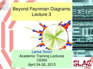
Beyond Feynman Diagrams Lecture 2 . Lance Dixon Academic Training Lectures CERN April 24-26, 2013. Modern methods for trees. Color organization (briefly) Spinor variables Simple examples Factorization properties BCFW ( on-shell) recursion relations.

Beyond Feynman Diagrams Lecture 2
E N D
Presentation Transcript
Beyond Feynman DiagramsLecture 2 Lance Dixon Academic Training Lectures CERN April 24-26, 2013
Modern methods for trees Color organization (briefly) Spinorvariables Simple examples Factorization properties BCFW (on-shell) recursion relations Lecture 2 April 25, 2013
How to organizegauge theory amplitudes • Avoid tangled algebra of color and Lorentz indices generated by Feynman rules structure constants • Take advantage of physical properties of amplitudes • Basic tools: • dual (trace-based) color decompositions • spinor helicity formalism Lecture 2 April 25, 2013
Color Standard color factor for a QCD graph has lots of structure constants contracted in various orders; for example: Write every n-gluon tree graph color factor as a sum of traces of matrices T a in the fundamental (defining) representation of SU(Nc): + all non-cyclic permutations Use definition: + normalization: Lecture 2 April 25, 2013
Double-line picture (’t Hooft) • In limit of large number of colors Nc, a gluon is always a combination of a color and a different anti-color. • Gluon tree amplitudes dressed by lines carrying color indices, 1,2,3,…,Nc. • Leads to color ordering of the external gluons. • Cross section, summed over colors of all external gluons • = S |color-ordered amplitudes|2 • Can still use this picture at Nc=3. • Color-ordered amplitudes are • still the building blocks. • Corrections to the color-summed • cross section, can be handled • exactly, but are suppressed by 1/ Nc2 Lecture 2 April 25, 2013
color-ordered subamplitudeonly depends on momenta. Compute separately for each cycliclyinequivalent helicity configuration • Because comes from planar diagrams • with cyclic ordering of external legs fixed to 1,2,…,n, • it only has singularities in cyclicly-adjacent channels si,i+1, … Trace-based (dual) color decomposition For n-gluontree amplitudes, the color decomposition is momenta helicities color Similar decompositions for amplitudes with external quarks. Lecture 2 April 25, 2013
Far fewer factorization channelswith color ordering 3 2 k+1 3 … 1 1 … k 16 n ( ) only n k partitions n 4 … … k+1 2 n-1 k+2 n k+2 Lecture 2 April 25, 2013
Color sums Parton model says to sum/average over final/initial colors (as well as helicities): Insert: and do color sums to get: • Up to 1/Nc2 suppressed effects, squared subamplitudes have definite color flow – importantfor development of parton shower Lecture 2 April 25, 2013
But for elementary particles with spin (e.g. all except Higgs!) there is a better way: Take “square root” of 4-vectorskim (spin 1) use Dirac (Weyl) spinorsua(ki) (spin ½) q,g,g, all have 2 helicity states, Spinor helicity formalism Scattering amplitudes for massless plane waves of definite momentum: Lorentz 4-vectors kim ki2=0 Natural to use Lorentz-invariant products (invariant masses): Lecture 2 April 25, 2013
Massless Dirac spinors Positive and negative energy solutions to the massless Dirac equation, are identical up to normalization. Chirality/helicityeigenstates are Explicitly, in the Dirac representation Lecture 2 April 25, 2013
Spinor products Instead of Lorentz products: Use spinor products: Identity These are complex square roots of Lorentz products (for real ki): Lecture 2 April 25, 2013
2 3 add helicity information, numeric labels R R 4 1 L L Fierz identity helicity suppressed as 1 || 3 or 2 || 4 ~ Simplest Feynman diagram of all g Lecture 2 April 25, 2013
Useful to rewrite answer Crossing symmetry more manifest if we switch to all-outgoing helicity labels (flip signs of incoming helicities) 2- 3+ useful identities: 1+ 4- “holomorphic” “antiholomorphic” Schouten Lecture 2 April 25, 2013
C 2+ 3+ 1- 4- P 2- 3- 2+ 3- 1+ 4+ 1- 4+ Symmetries for all other helicity config’s 2- 3+ 1+ 4- Lecture 2 April 25, 2013
Unpolarized, helicity-summed cross sections (the norm in QCD) Lecture 2 April 25, 2013
Helicity formalism for massless vectors Berends, Kleiss, De Causmaecker, Gastmans, Wu (1981); De Causmaecker, Gastmans, Troost, Wu (1982); Xu, Zhang, Chang (1984); Kleiss, Stirling (1985); Gunion, Kunszt (1985) obeys (required transversality) (bonus) under azimuthal rotation about ki axis, helicity +1/2 helicity -1/2 so as required for helicity +1 Lecture 2 April 25, 2013
Next most famous pair of Feynman diagrams (to a higher-order QCD person) g g Lecture 2 April 25, 2013
Choose to remove 2nd graph (cont.) Lecture 2 April 25, 2013
Properties of 1. Soft gluon behavior Universal “eikonal” factors for emission of soft gluon s between two hard partons a and b Soft emission is from the classical chromoelectric current: independent of partontype (q vs. g) and helicity – only depends on momenta of a,b, and color charge: Lecture 2 April 25, 2013
Universal collinear factors, or splitting amplitudes depend on partontype and helicity (cont.) Properties of 2. Collinear behavior Square root of Altarelli-Parisi splitting probablility z 1-z Lecture 2 April 25, 2013
Maximally helicity-violating (MHV) amplitudes: 1 2 = Parke-Taylor formula (1986) (i-1) Simplest pure-gluonic amplitudes Note: helicity label assumes particle is outgoing; reverse if it’s incoming Strikingly, many vanish: Lecture 2 April 25, 2013
MHV amplitudes with massless quarks Helicity conservation on fermion line more vanishing ones: the MHV amplitudes: Related to pure-gluon MHV amplitudes by a secret supersymmetry: after stripping off color factors, massless quarks ~gluinos Grisaru, Pendleton, van Nieuwenhuizen (1977); Parke, Taylor (1985); Kunszt (1986); Nair (1988) Lecture 2 April 25, 2013
2. Gluoniccollinear limits: So and plus parity conjugates Properties of MHV amplitudes 1. Soft limit Lecture 2 April 25, 2013
scalars gauge theory angular momentum mismatch Spinor Magic Spinor products precisely capture square-root + phase behavior in collinear limit. Excellent variables for helicity amplitudes Lecture 2 April 25, 2013
Utility of Complex Momenta i- k+ • Makes sense of most basic process: all 3 particles massless j- real (singular) complex (nonsingular) use conjugate kinematics for (++-): Lecture 2 April 25, 2013
Tree-level “plasticity” BCFW recursion relations • BCFW consider a family of on-shell amplitudes An(z) depending on a complex parameter zwhich shifts the momenta to complex values • For example, the [n,1›shift: • On-shell condition: similarly, • Momentum conservation: Lecture 2 April 25, 2013
Cauchy: Analyticity recursion relations meromorphic function, each pole corresponds to one factorization Where are the poles? Require on-shell intermediate state, Lecture 2 April 25, 2013
Final formula Britto, Cachazo, Feng, hep-th/0412308 Ak+1 and An-k+1 are on-shellcolor-ordered tree amplitudes with fewer legs, evaluated with 2momenta shifted by a complex amount Lecture 2 April 25, 2013
To finish proof, show Britto, Cachazo, Feng, Witten, hep-th/0501052 Propagators: 3-point vertices: Polarization vectors: Total: Lecture 2 April 25, 2013
MHV example • Apply the [n,1›BCFW formula to the MHV amplitude • The generic diagram vanishes because 2 + 2 = 4 > 3 • So one of the two tree amplitudes is always zero • The one exception is k = 2, which is different because - + Lecture 2 April 25, 2013
MHV example (cont.) • For k = 2, we compute the value of z: • Kinematics are complex collinear • The only term in the BCFW formula is: Lecture 2 April 25, 2013
MHV example (cont.) • Using one confirms • This proves the Parke-Taylor formula by induction on n. Lecture 2 April 25, 2013
Parke-Taylor formula Initial data Lecture 2 April 25, 2013
3 BCF diagrams related by symmetry A 6-gluon example 220 Feynman diagrams for gggggg Helicity + color + MHV results + symmetries Lecture 2 April 25, 2013
The one diagram Lecture 2 April 25, 2013
Simpler than form found in 1980s despite (because of?) spurious singularities Mangano, Parke, Xu (1988) Simple final form Relative simplicity muchmore striking for n>6 Lecture 2 April 25, 2013