Download
1 / 22
220 likes | 356 Vues
Fast Moment Estimation in Data Streams in Optimal Space. Daniel Kane, Jelani Nelson, Ely Porat, David Woodruff Harvard MIT Bar-Ilan IBM. l p -estimation: Problem Statement. Model x = (x 1 , x 2 , …, x n ) starts off as 0 n

E N D
Fast Moment Estimation in Data Streams in Optimal Space Daniel Kane, Jelani Nelson, Ely Porat, David Woodruff Harvard MIT Bar-Ilan IBM
lp-estimation: Problem Statement • Model • x = (x1, x2, …, xn) starts off as 0n • Stream of m updates (j1, v1), …, (jm, vm) • Update (j, v) causes change xj = xj + v • v 2 {-M, -M+1, …, M} • Problem • Output lp = j=1n |xj|p = |x|p • Want small space and fast update time • For simplicity: n, m, M are polynomially related
Some Bad News • Alon, Matias, and Szegedy • No sublinear space algorithms unless • Approximation (allow output to be (1±ε) lp) • Randomization (allow 1% failure probability) • New goal • Output (1±ε) lp with probability 99%
Some More Bad News • Estimating lp for p > 2 in a stream requires n1-2/p space [AMS, IW, SS] • We focus on the “feasible” regime, when p 2 (0,2) p = 0 and p = 2 well-understood • p = 0 is number of distinct elements • p = 2 is Euclidean norm
b1 b2 … bn Query point a 2 Rd Database points Applications for p 2 [1,2) Can quickly replace d-dimensional points with small sketches lp-norm for p 2 [1,2) less sensitive to outliers • Nearest neighbor • Regression • Subspace approximation Want argminj |a-bj|p Less likely to be spoiled by noise in each coordinate
Applications for p 2 (0,1) Best entropy estimation in a stream [HNO] • Empirical entropy = j qj log(1/qj), where qj = |xj|/|x|1 • Estimates |x|p for O(log 1/ε) different p 2 (0,1) • Interpolates a polynomial through these values to estimate entropy • Entropy used for detecting DoS attacks, etc.
Previous Work for p 2 (0,2) • Lot of players • FKSV, I, KNW, GC, NW, AOK • Tradeoffs possible • Can get optimal ε-2 log n bits of space, but then the update time is at least 1/ε2 • BIG difference in practice between ε-2update time and O(1) (e.g., AMS vs. TZ for p = 2) • No way to get close to optimal space with less than poly(1/ε) update time
Our Results • For every p 2 (0,2) • estimate lp with optimal ε-2 log n bits of space • log2 1/ε log log 1/ε update time • exponential improvement over previous update time • For entropy • Exponential improvement over previous update time (polylog 1/ε versus poly 1/ε)
Our Algorithm Split coordinates into “head” and “tail” j 2 “head” if |xj|p¸ε2 |x|pp j2 “tail” if |xj|p < ε2 |x|pp Estimate |x|pp = |xhead|pp + |xtail|pp separately Two completely different procedures
Outline • Estimating |xhead|pp • Estimating |xtail|pp • Putting it all together
Simplifications We can assume we know the set of “head” coordinates, as well as their signs • Can be found using known algorithms [CountSketch] Challenge • Need j in head |xj|p
We DO NOT • maintain sum of values in each cell • We DO NOT • maintain the inner product of values in a cell with a random sign vector Key idea: for each cell c, if S is the set of items hashed to c, let V(c) = j in S xj¢ exp(2¼i h(j)/r ) r is a parameter, i = sqrt(-1) Estimating |xhead|p p xj log 1/ε rows 1/ε2 columns Hash each coordinate to a unique column in each row
Our Algorithm To estimate |xhead|pp • For each j in the head, find an arbitrary cell c(j) containing j and no other head coordinates • Compute yj = sign(xj) ¢ exp(-2¼i h(j)/r) ¢ V(c) • Recall V(c) = j in S xj¢ exp(2¼i h(j)/r ) • Expected value of yj is |xj| • What can we say about yjp? • What does it mean?
Our Algorithm • Recall yj = sign(xj) ¢ exp(-2¼i h(j)/r) ¢ V(c) • What is yj1/2 if yj = -4? • -4 = 4 exp(¼ i) • (-4)1/2 = 2 exp(¼ i / 2) = 2i or 2 exp(- ¼ i / 2) = -2i • By yjp we mean |yj|p exp(i p arg(z)), where arg(z) 2 (-¼, ¼] is the angle of yj in the complex plane
Our Algorithm Wishful thinking • Estimator = j in head yjp • Intuitively, when p = 1, since E[yj] = |yj| we have an unbiased estimator • For general p, this may be complex, so how about Estimator = Re [j in head yjp]? • Almost correct, but we want optimal space, and we’re ignoring most of the cells • Better: yj = Meancells c isolating j sign(xj) ¢ exp(-2¼i h(j)/r)¢V(c)
Analysis • Why did we use roots of unity? • Estimator is real part of j in head yjp • j in head yjp = j in head |yj|p¢ (1+zj)p for zj = (yj - |yj|)/|yj| • Can apply Generalized Binomial theorem • E[|yj|p (1+zj)p] = |yj|p¢k=01{p choose k} E[zjk] = |yj|p + small since E[zjk] = 0 if 0 < k < r Generalized binomial coefficient {p choose k} = p ¢ (p-1) (p-k+1)/k! = O(1/k1+p) Intuitively variance is small because head coordinates don’t collide
Outline • Estimating |xhead|pp • Estimating |xtail|pp • Putting it all together
Our Algorithm Estimating |xtail|pp xj • In each bucket b maintain an unbiased estimator of the • p-th power of the p-norm |x(b)|pp in the bucket [Li] • If Z1, …, Zs are p-stable, for any vector a = (a1, …, as), • j=1s Zj¢aj» |a|p Z, for Z also p-stable • Add up estimators in all buckets not containing a head • coordinate (variance is small)
Outline • Estimating |xhead|pp • Estimating |xtail|pp • Putting it all together
Complexity Bag of tricks Example • For optimal space, in buckets in the light estimator, we prove 1/εp – wise independent p-stable variables suffice • Rewrite Li’s estimator so that [KNW] can be applied • Need to evaluate a degree- 1/εppolynomial per update • Instead: batch 1/εpupdates together and do fast multipoint evaluation • Can be deamortized • Use that different buckets are pairwise independent
Complexity Example # 2 • Finding head coordinates requires ε-2 log2 n space • Reduce the universe size to poly 1/ε by hashing • Now requires ε-2 log n log 1/ε space • Replace ε with ε log1/2 1/ε • Head estimator okay, but slightly adjust light estimator
Conclusion • For every p 2 (0,2) • estimate lp with optimal ε-2 log n bits of space • log2 1/ε log log 1/ε update time • exponential improvement over previous update time • For entropy • Exponential improvement over previous update time (polylog 1/ε versus poly 1/ε)