Nonlinear Model Predictive Control using Automatic Differentiation
Nonlinear Model Predictive Control using Automatic Differentiation. Yi Cao Cranfield University, UK. Outline. Computation in MPC Dynamic Sensitivity using AD Nonlinear Least Square MPC Error Analysis and Control Evaporator Case Study Performance Comparison Conclusions.


Nonlinear Model Predictive Control using Automatic Differentiation
E N D
Presentation Transcript
Nonlinear Model Predictive Control using Automatic Differentiation Yi Cao Cranfield University, UK Colloquium on Predictive Control, Sheffield
Outline • Computation in MPC • Dynamic Sensitivity using AD • Nonlinear Least Square MPC • Error Analysis and Control • Evaporator Case Study • Performance Comparison • Conclusions Colloquium on Predictive Control, Sheffield
Computation in Predictive Control • Predictive control: at tk, calculate OC for tk· t· tk+P, apply only u(tk), repeat at tk+1 • Prediction: online solving ODE • Optimization: repeat prediction, sensitivity required. • Typically, over 80% time spend on solving ODE + sensitivity Colloquium on Predictive Control, Sheffield
Current Status • Linear MPC successfully used in industry • Most systems are nonlinear. NMPC desired. • Computation: solving ODE and NLP online. • Difficult to get gradient for large ODE systems. • Finite difference: inefficient and inaccurate • Sensitivity equation: n×m ODE’s • Adjoint system: TPB problem • Other methods: sequential linearization and orthogonal collocation Colloquium on Predictive Control, Sheffield
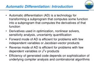
Automatic Differentiation • Limitation of finite and symbolic difference • Function = sequence of fundamental OP • Derivatives of fundamental OP are known • Numerically apply chain rules • Basic modes: forward and reverse • Implementation: • operating overloading • Source translation Colloquium on Predictive Control, Sheffield
ODE and Automatic Differentiation • z(t)=f(x), x(t)=x0+x1t+x2t2+…+xdtd • z(t)=z0+z1t+z2t2+…+zdtd • AD forward: zk = zk(x0,x1,…,xk) • AD reverse: zk /xj = zk-j / x0 = Ak-j • f’(x)=A0+A1t++Adtd • ODE: dx/dt=f(x), dx/dt=z(t), xk+1=zk/(k+1). • x0=x(t0), x1=z0(x0), x2=z1(x0,x1), … • Sensitivity: Bk=dxk/dx0=1/kki=0 Ak-i-1Bi, B0=I • dB/dt=f’(x), B=B0+B1t++Bdtd • x(t0+1)=di=0 xi, dx(t0+1)/dx0=di=0Bi Colloquium on Predictive Control, Sheffield
Non-autonomous Systems I • For control systems: dx/dt=f(x,u) • u(t)=u0+u1t+u2t2+…+udtd • (x0, u(t)) → x(t), dx(t)/duk=? • Method I: Augmented system: • dv1/dt=v2, …, dvd+1/dt=0, vk+1(t0)=uk, u=v1 • X=[xT vT]T, dX/dt=F(X) (autonomous) • High dimension system, n+md • Not suitable for systems with large m Colloquium on Predictive Control, Sheffield
Non-autonomous Systems II • Method II: nonsquare AD • Let v=[u0T, u1T, …, udT]T • xk+1 = zk(x0,x1,…,xk,v)/(k+1) • Ak=[Akx | Akv] := [zk/x0 | zk/v] • Bk=[Bkx | Bkv] := [dxk/dx0 | dxk/dv] • Bk = Ak-1+k-1j=1A(k-j-1)xBj, B0=[I | 0] • x(t0+1)=dk=0xk, • dx(t0+1)/dv= dk=0Bkv ,dx(t0+1)/dx(t0)= dk=0Bkx Colloquium on Predictive Control, Sheffield
Nonlinear Least Square MPC • Φ=½∑Pk=0(x(tk)-rk)TWk(x(tk)-rk) s.t. dx/dt=f(x,u,d), t[t0, tP], x(t0) given, uj=u(tj)=u(t), t[tj, tj+1], uj=uM-1, j[M, P-1], L≤u≤V, scale t=tj+1-tj=1. • Nonlinear LS: minL≤U≤VΦ=½E(U)TE(U) • Jacobian: J(U)=∂E/∂U • Gradient: G(U)=JT(U)E(U) • Hessian: H(U)=JT(U)J(U)+Q(U)≈JT(U)J(U) Colloquium on Predictive Control, Sheffield
ODE and Jacobian using AD • Efficient algorithm requires efficient J(U) • Difficult: E(U) is nonlinear dynamic • Ji,j=Wi½dx(ti)/duj-1 for i≥j, otherwise, Ji,j=0 • Algorithm: for k=0:P-1, x0=x(tk) • Forward AD: xi, i=1,…,d, → x(tk+1) • Reverse AD: Aix, Aiu • Accumulate: Bix, Biu, → Bu(k)=Biu, Bx(k)=Bix • J(k+1)j=Wk+1½Bx(k)…Bx(j)Bu(j-1), j=1,…,k+1 • K=k+1 Colloquium on Predictive Control, Sheffield
NLS MPC using AD • Collect information: x, d, r, etc. • Nonlinear LS to give a guess u • Solve ODE and calculate J • Update u and check convergence • Implement the first move Colloquium on Predictive Control, Sheffield
Error Analysis • Taylor coefficients by AD is accurate. • x(tk)= xk has truncation error, ek (local). • ek will propagated to k+1, …, P (global). • Local error controllable by order and step • Global error depend on sensitivity dxk1/dxk • Remainder: k≈C(h/r)k+1 • Convergence radius: r ≈ rk=|xk-1|/|xk| • k-1=k(r/h)=k+|xk| →k=|xk|/(r/h-1) Colloquium on Predictive Control, Sheffield
Error Control • Tolerance < d • Increase order, d or decrease step, h? • Decrease h by h/c (c>1): =d(1/c)d+1 • c=(d/)1/(d+1) , increase op by factor c • Increase d to d+p (p>0): =d(h/r)p • p=ln(/)/ln(h/r), increase op by (1+p/d)2 • c<(1+p/d)2 decrease h, • otherwise increase d Colloquium on Predictive Control, Sheffield
Case Study • Evaporator process • 3 measurable states: L2, X2 and P2 • 3 manipulates: 0≤F2≤4, 0≤P100,F200≤400 • Set point change: X2 from 25% to 15% P2 from 50.5 kPa to 70 kPa • Disturbance: F1, X1, T1 and T200 20% • All disturbance unmeasured. • T=1 min, M=5 min, P=10 min, W=[100,1,1] Colloquium on Predictive Control, Sheffield
Simulation Results Colloquium on Predictive Control, Sheffield
Performance Comparison • CVODES, a state-of-the-art solver for dynamic sensitivity. • Simultaneously solves ODE and sensitivity • Two approaches: full & partial integration. • Three approaches programmed in C • Tested on Windows XP P-IV 2.5GHz • Solve evaporator ODE + sensitivity using input generated by NMPC. Colloquium on Predictive Control, Sheffield
Accuracy and Efficiency Colloquium on Predictive Control, Sheffield
Conclusions • AD can play an important role to improve nonlinear model predictive control • Efficient algorithm to integrate ODE at the same time to calculate sensitivity • Error analysis and control algorithm • Efficiency validated via comparison with state-of-the-art software. • Satisfactory performance with Evaporator study Colloquium on Predictive Control, Sheffield