Download
1 / 26
260 likes | 539 Vues
Estimation Methods for Dose-response Functions Bahman Shafii Statistical Programs College of Agricultural and Life Sciences University of Idaho, Moscow, Idaho. Introduction. Dose-response models are common in agricultural research. They can encompass many types of problems:.

E N D
Estimation Methods for Dose-response Functions Bahman Shafii Statistical Programs College of Agricultural and Life Sciences University of Idaho, Moscow, Idaho
Introduction • Dose-response models are common in agricultural research. • They can encompass many types of problems: • Time effects • germination, emergence, hatching • exposure times • Environmental effects • temperature exposure • chemical exposure • depth or distance from exposure • Related Problems - Bioassay • standard curves and determination of unknown quantities
The response distribution: • Continuous • Normal • Log Normal • Gamma, etc. • Discrete - quantal responses • Binomial, Multinomial (yes/no) • Poisson (count)
Response Response Dose Dose • The response form: • Typically expressed as a nonlinear curve • increasing or decreasing sigmoidal form • increasing or decreasing asymptotic form
Estimation • Curve estimation. • Linear or non-linear techniques. • Estimate other quantities: • percentiles. • typically: LD50, LC50, EC50, etc. • percentileestimation problematic. • inverted solutions. • unknown distributions. • approximate variances.
Objectives • Outline estimation methods for dose- • response models. • Traditional approaches. • Probit - Least Squares. • Modern approaches. • Probit - Maximum Likelihood • Generalized non-linear models. • Bayesian solutions.
Methods • where • pij = yij / N and yij is the number of successes out of N • trials in the jth replication of the ith dose. • b0 and b1 are regression parameters and ei is a random • error; eij ~ N(0,s2). • Minimize: SSerror = (pij - probit)2 ^ • Traditional Approach • Probit Analysis - Least Squares • A linearized least squares estimation (Bliss, 1934 ; Fisher, 1935; • Finney, 1971): • Probiti = F -1(pij) = b0 + b1*dosei + eij (1)
• is a convenient CDF form or “tolerance • distribution“, e.g. • Normal:pij = (1/2) exp((x-)2/2 • Logistic:pij = 1 / (1 + exp( -b1( dosei - b0 )) • Modified Logistic:pij = C + (C-M) / (1 + exp( -b1(dosei -b0)) • (e.g. Seefeldt et al. 1995) • Gompertz: pij = b0 (1 - exp(exp(-b1(dose)))) • Exponential:pij = b0 exp(-b1(dose)) • SAS: PROC REG.
Modern Approach • Probit Analysis - Maximum Likelihood • The responses, yij, are assumed binomial at each dose i • with parameter pi. Using the joint likelihood, L(pi) : • Maximize: L(pi) P (pi)yij (1 - pi)(N - yij) (2) • for data set yij where pi = F (b0 + b1*dosei ) and b0, b1, • and dosei are those given previously. • The CDF, F, is typically defined as a Normal, Logistic, or • Gompertz distribution as given above. • SAS: PROC PROBIT.
Probit Analysis • Limitations: • Least squares limited. • Linearized solution to a non-linear problem. • Even under ML, solution for percentiles approximated. • inversion. • use of the ratio b0/b1 (Fieller, 1944). • Appropriate only for proportional data. • Assumes the response F-1(pij) ~ N(m, s2). • Interval estimation and comparison of percentile • values approximated.
Modern Approaches (cont) • Nonlinear Regression - IterativeLeast Squares • Directly models the response as: • yij = f(dosei) + eij (3) • where yij is an observed continuous response, f(dosei) • may be generalized to any continuous function of dose • and eij ~ N(0, s2). • Minimize: SSerror = [ yij - f(dosei) ]2. • SAS: PROC NLIN.
Nonlinear Regression - Iterative Least Squares • Limitations: • assumes the data, yij , is continuous; could be discrete. • the response distribution may not be Normal, • i.e.eij ~ N(0, s2). • standard errors and inference are asymptotic. • treatment comparisons difficult in SAS. • differential sums of squares. • specialized SAS codes ; PROC IML.
Modern Approaches (cont) • Generalized Nonlinear Model - Maximum Likelihood • Directly models the response as: • yij = f(dosei) + eij • where yij and f(dosei) are as defined above. • Estimation through maximum likelihood where the • response distribution may take on many forms: • Normal: yij ~ N(i, ) , • Binomial: yij ~ bin(N, pi) , • Poisson: yij ~ poisson(i) , or • in general: yij ~ ƒ().
Generalized Nonlinear Model - Maximum Likelihood • Maximize: L() Pƒ( | yij) (4) • Nonlinear estimation. • Response distribution not restricted to Normal. • May also incorporate random components into the model. • Treatment comparisons easier in SAS. • Contrast and estimate statements. • SAS: PROC NLMIXED.
Generalized Non-linear Model - Inference • Formulate a full dummy variable model encompassing k • treatments. • The joint likelihood over the k treatments becomes: • L(k) Pijkƒ(k | yijk) (5) • where yijk is the jth replication of the ith dose in the kth • treatment and qk are the parameters of the kth treatment. • Comparison of parameter values is then possible through • single and multiple degree of freedom contrasts.
Generalized Nonlinear Model • Limitations • percentile solution may still be based on inversion or • Fieller’s theorem. • inferences based on normal theory approximations. • standard errors and confidence intervals asymptotic.
Modern Approaches (cont) • Bayesian Estimation - Iterative Numerical Techniques • Considers the probability of the parameters, q, • given the data yij. • Using Bayes theorem, estimate: • p(q|yij) = p(yij|q)*p(q) (6) • p(yij|q)*p(q)dq where p(q|yij) is the posterior distribution of q given the data yij, p(yij|q) is the likelihood defined above, and p(q) is a prior probability distribution for the parameters q.
Bayesian Estimation - Iterative Numerical Techniques • Nonlinear estimation. • Percentiles can be found from the distribution of q. • The likelihood is same as Generalized Nonlinear Model. • flexibility in the response distribution. • f(dosei) any continuous funtion of dose. • Inherently allows updating of the estimation. • Correct interval estimation (credible intervals). • agrees well with GNLM at midrange percentiles. • can perform better at extreme percentiles. • SAS: No procedure available.
Bayesian Estimation - Iterative Numerical Techniques • Limitations • User must specify a prior probability p(q). • Estimation requires custom programming. • SAS: Datastep, PROC IML • Custom C program codes • Specialized software: WinBUGS • Computationally intensive solutions. • Requires statistical expertise. • Sample programs and data are available at: • http://www.uidaho.edu/ag/statprog
Concluding Remarks • Dose-response models have wide application in agriculture. • They are useful for quantifying the relative efficacy of various • treatments. • Probit models are limited in scope. • Generalized nonlinear and Bayesian models provide the most • flexible framework for estimating dose-response. • Can use various response distributions • Can use various dose-response models. • Can incorporate random model effects. • Can be used to compare treatments. • GNLM: full dummy variable modeling. • Bayesian methods: probability statements.
Concluding Remarks • Both GNLM and Bayesian methods give similar percentile • estimates for midrange percentiles. • Generalized nonlinear models sufficient in most situations. • Software available. • Bayesian estimation is preferred when estimating extreme • percentiles. • Custom programming required.
References • Bliss, C. I. 1934. The method of probits. Science, 79:2037, 38-39 • Bliss, C. I. 1938. The determination of dosage-mortality curves from small • numbers. Quart. J. Pharm., 11: 192-216. • Berkson, J. 1944.Application of the Logistic function to bio-assay. J. • Amer. Stat. Assoc. 39: 357-65. • Feiller, E. C. 1944. A fundamental formula in the statistics of biological • assay and some applications. Quart. J. Pharm. 17: 117-23. • Finney, D. J. 1971. Probit Analysis. Cambridge University Press, London. • Fisher, R. A. 1935. Appendix to Bliss, C. I.: The case of zero survivors., • Ann. Appl. Biol., 22: 164-5. • SAS Inst. Inc. 2004. SAS OnlineDoc, Version 9, Cary, NC. • Seefeldt, S.S., J. E. Jensen, and P. Fuerst. 1995. Log-logistic analysis of • herbicide dose-response relationships. Weed Technol. 9:218-227.
“Top Ten Things A Statistician Does Not Want to Hear” 10. I have never had a course in statistics, but how hard can it be? 9. I don’t have a design! 8. I should have talked to you before I ran the experiment, but..... 7. Why should I replicate? I might get a different answer! 6. I should have randomized what?
“Top Ten Things A Statistician Does Not Want to Hear” 5. Could you have this by tomorrow? 4. Halfway through the experiment, we changed..... 3. Can you make it so that the p-value is less than.....? 2. I have 20,000 observations from this one cow! 1. Do you have a minute? Thank you!