Enhancing Molecular Science Productivity with NWChem: A Comprehensive Overview
610 likes | 753 Vues
NWChem, developed by Oak Ridge National Laboratory with funding from the U.S. Department of Energy, offers cutting-edge modeling and simulation capabilities for molecular science. This computational chemistry package supports a wide range of molecules, including biomolecules, and features advanced electronic structure calculations, molecular dynamics, and solid-state capabilities. With scalable performance on thousands of processors and easy access for developers through a Python interface, NWChem serves over 1000 global installations, making significant contributions to research in chemistry and related fields.

Enhancing Molecular Science Productivity with NWChem: A Comprehensive Overview
E N D
Presentation Transcript
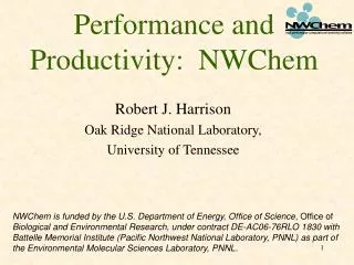
Performance and Productivity: NWChem Robert J. Harrison Oak Ridge National Laboratory, University of Tennessee NWChem is funded by the U.S. Department of Energy, Office of Science, Office of Biological and Environmental Research, under contract DE-AC06-76RLO 1830 with Battelle Memorial Institute (Pacific Northwest National Laboratory, PNNL) as part of the Environmental Molecular Sciences Laboratory, PNNL.
NWChem Citation T.H. Dunning, Jr., D.A. Dixon, M.F. Guest R. J. Harrison, J. A. Nichols, T. P. Straatsma, M. Dupuis,E. J. Bylaska, G. I. Fann, T. L. Windus, E. Apra, W. de Jong,S. Hirata, M. T. Hackler, J. Anchell, D. Bernholdt, P. Borowski,T. Clark, D. Clerc, H. Dachsel, M. Deegan, K. Dyall, D. Elwood,H. Fruchtl, E. Glendening, M. Gutowski, K. Hirao, A. Hess,J. Jaffe, B. Johnson, J. Ju, R. Kendall, R. Kobayashi, R. Kutteh,Z. Lin, R. Littlefield, X. Long, B. Meng, T. Nakajima,J. Nieplocha, S. Niu, M. Rosing, G. Sandrone, M. Stave, H. Taylor,G. Thomas, J. van Lenthe, K. Wolinski, A. Wong, and Z. Zhang, "NWChem, A Computational Chemistry Package for Parallel Computers, Version 4.1" (2002), Pacific Northwest National Laboratory,Richland, Washington 99352-0999, USA.
NWChem Overview • Provides major new modeling and simulation capability for molecular science • Broad range of molecules, including biomolecules • Electronic structure of molecules (non-relativistic, relativistic, one-/two-component, ECPs, second deriv.) • Increasingly extensive solid state capability • Molecular dynamics, molecular mechanics • Extensible and long-lived • Freely distributed – installed at about 1000 sites worldwide • Performance characteristics – designed for MPP • Single node performance comparable to best serial codes • Scalability to 1000’s of processors • Portable – runs on a wide range of computers
Molecular Science Software Suite (MS3) http://www.emsl.pnl.gov/pub/docs/ecce/ http://www.emsl.pnl.gov/pub/docs/nwchem/ http://www.emsl.pnl.gov/pub/docs/parsoft/
NWChem to go ... Compaq iPAQ Linux (Intimate) 64 Mbyte RAM, 16 Mbyte flash, 2 Gbyte PCMCIA disk Strongarm CPU Sadly, no FPU
Higher-level composition • Modular, hierarchical design • Easy to access high level features • Easy to extend with new high level features • Standardized interfaces • Reuse of low-level functionality without side effects • Distributed-shared memory parallel programming model • Non-uniform memory access (NUMA) aware algorithms • Python interface • User’s & developers can write NWChem programs in Python • Cool stuff – now becoming available • Automatic code generation – compose with many-body theory and/or tensor expressions (already in NWChem 4.5) • Multiresolution quantum chemistry – compose with operators and functions
Generic Tasks Energy, structure, … SCF energy, gradient, … Molecular Calculation Modules DFT energy, gradient, … MD, NMR, Solvation, … Optimize, Dynamics, … Run-time database Molecular Modeling Toolkit Basis Set Object Geometry Object Integral API PeIGS ... ... Molecular Software Development Toolkit Parallel IO Memory Allocator Global Arrays NWChem Architecture • Object-oriented design • abstraction, data hiding, APIs • Parallel programming model • non-uniform memory access, global arrays, MPI • Infrastructure • GA, Parallel I/O, RTDB, MA, ... • Program modules • communication only through the database • persistence for easy restart
Issues in Parallel Computing • Expressing and managing concurrency • The memory hierarchy • Efficient sequential execution
The Memory Hierarchy • Non-uniform memory access - NUMA • Your workstation is NUMA - registers, cache, main memory, virtual memory • Parallel computers just add non-local memory(s) • Unites sequential and parallel computation • Differ only in expression and management of concurrency • Distributed data • Do not limit calculation by resources of one node • Exploit aggregate resources of the whole machine • SCF and DFT can distribute all data > O(N) • MP2 gradients distribute all data > O(N2)
J. Nieplocha Supported by DOE/ASCR/MICS Shared-memory-like model Fast local access NUMA aware and easy to use MIMD and data-parallel modes Inter-operates with MPI, … BLAS and linear algebra interface Used by most major chemistry codes, also in financial futures forecasting, astrophysics, computer graphics, … Ported to major parallel machines IBM, Cray, SGI, clusters, ... Physically distributed data Single, shared data structure Parallel Programming ModelGlobal Arrays + MPI http://www.emsl.pnl.gov/pub/docs/global
Non-uniform memory access model of computation Shared Object Shared Object 1-sided communication 1-sided communication copy to shared object copy to local memory compute/update local memory local memory local memory
O(1) programmers … O(1000) nodes …O(100,000) processors … O(10,000,000) threads • Expressing/managing concurrency at the petascale • It is too trite to say that the parallelism is in the physics • Must express and discover parallelism at more levels • Low level tools (MPI, Co-Array Fortran, UPC, …) don’t discover parallelism or hide complexity or facilitate abstraction • Management of the memory hierarchy • Sending data from one multiprocessor chip to another will be like us taking a trip to Europe • Memory will be deeper ; less uniformity between vendors • Need tools to automate and manage this, even at runtime
Synthesis of High Performance Algorithms for Electronic Structure Calculations • Sadayappan, Baumgartner, Cociorva, Pitzer (OSU) Ramanujam (LSU)Bernholdt, Dean, White III, Harrison (ORNL)Hirata (PNNL)Nooijen (Waterloo) • Objective: • Automate the implementation of optimized parallel computer programs for many-electron methods expressed as tensor contractions • Multi-disciplinary, multi-institution project • Collaboration between NSF ITR, DOE SciDAC, and ORNL LDRD projects
CCSD Doubles Equation hbar[a,b,i,j] == sum[f[b,c]*t[i,j,a,c],{c}] -sum[f[k,c]*t[k,b]*t[i,j,a,c],{k,c}] +sum[f[a,c]*t[i,j,c,b],{c}] -sum[f[k,c]*t[k,a]*t[i,j,c,b],{k,c}] -sum[f[k,j]*t[i,k,a,b],{k}] -sum[f[k,c]*t[j,c]*t[i,k,a,b],{k,c}] -sum[f[k,i]*t[j,k,b,a],{k}] -sum[f[k,c]*t[i,c]*t[j,k,b,a],{k,c}] +sum[t[i,c]*t[j,d]*v[a,b,c,d],{c,d}] +sum[t[i,j,c,d]*v[a,b,c,d],{c,d}] +sum[t[j,c]*v[a,b,i,c],{c}] -sum[t[k,b]*v[a,k,i,j],{k}] +sum[t[i,c]*v[b,a,j,c],{c}] -sum[t[k,a]*v[b,k,j,i],{k}] -sum[t[k,d]*t[i,j,c,b]*v[k,a,c,d],{k,c,d}] -sum[t[i,c]*t[j,k,b,d]*v[k,a,c,d],{k,c,d}] -sum[t[j,c]*t[k,b]*v[k,a,c,i],{k,c}] +2*sum[t[j,k,b,c]*v[k,a,c,i],{k,c}] -sum[t[j,k,c,b]*v[k,a,c,i],{k,c}] -sum[t[i,c]*t[j,d]*t[k,b]*v[k,a,d,c],{k,c,d}] +2*sum[t[k,d]*t[i,j,c,b]*v[k,a,d,c],{k,c,d}] -sum[t[k,b]*t[i,j,c,d]*v[k,a,d,c],{k,c,d}] -sum[t[j,d]*t[i,k,c,b]*v[k,a,d,c],{k,c,d}] +2*sum[t[i,c]*t[j,k,b,d]*v[k,a,d,c],{k,c,d}] -sum[t[i,c]*t[j,k,d,b]*v[k,a,d,c],{k,c,d}] -sum[t[j,k,b,c]*v[k,a,i,c],{k,c}] -sum[t[i,c]*t[k,b]*v[k,a,j,c],{k,c}] -sum[t[i,k,c,b]*v[k,a,j,c],{k,c}] -sum[t[i,c]*t[j,d]*t[k,a]*v[k,b,c,d],{k,c,d}] -sum[t[k,d]*t[i,j,a,c]*v[k,b,c,d],{k,c,d}] -sum[t[k,a]*t[i,j,c,d]*v[k,b,c,d],{k,c,d}] +2*sum[t[j,d]*t[i,k,a,c]*v[k,b,c,d],{k,c,d}] -sum[t[j,d]*t[i,k,c,a]*v[k,b,c,d],{k,c,d}] -sum[t[i,c]*t[j,k,d,a]*v[k,b,c,d],{k,c,d}] -sum[t[i,c]*t[k,a]*v[k,b,c,j],{k,c}] +2*sum[t[i,k,a,c]*v[k,b,c,j],{k,c}] -sum[t[i,k,c,a]*v[k,b,c,j],{k,c}] +2*sum[t[k,d]*t[i,j,a,c]*v[k,b,d,c],{k,c,d}] -sum[t[j,d]*t[i,k,a,c]*v[k,b,d,c],{k,c,d}] -sum[t[j,c]*t[k,a]*v[k,b,i,c],{k,c}] -sum[t[j,k,c,a]*v[k,b,i,c],{k,c}] -sum[t[i,k,a,c]*v[k,b,j,c],{k,c}] +sum[t[i,c]*t[j,d]*t[k,a]*t[l,b]*v[k,l,c,d],{k,l,c,d}] -2*sum[t[k,b]*t[l,d]*t[i,j,a,c]*v[k,l,c,d],{k,l,c,d}] -2*sum[t[k,a]*t[l,d]*t[i,j,c,b]*v[k,l,c,d],{k,l,c,d}] +sum[t[k,a]*t[l,b]*t[i,j,c,d]*v[k,l,c,d],{k,l,c,d}] -2*sum[t[j,c]*t[l,d]*t[i,k,a,b]*v[k,l,c,d],{k,l,c,d}] -2*sum[t[j,d]*t[l,b]*t[i,k,a,c]*v[k,l,c,d],{k,l,c,d}] +sum[t[j,d]*t[l,b]*t[i,k,c,a]*v[k,l,c,d],{k,l,c,d}] -2*sum[t[i,c]*t[l,d]*t[j,k,b,a]*v[k,l,c,d],{k,l,c,d}] +sum[t[i,c]*t[l,a]*t[j,k,b,d]*v[k,l,c,d],{k,l,c,d}] +sum[t[i,c]*t[l,b]*t[j,k,d,a]*v[k,l,c,d],{k,l,c,d}] +sum[t[i,k,c,d]*t[j,l,b,a]*v[k,l,c,d],{k,l,c,d}] +4*sum[t[i,k,a,c]*t[j,l,b,d]*v[k,l,c,d],{k,l,c,d}] -2*sum[t[i,k,c,a]*t[j,l,b,d]*v[k,l,c,d],{k,l,c,d}] -2*sum[t[i,k,a,b]*t[j,l,c,d]*v[k,l,c,d],{k,l,c,d}] -2*sum[t[i,k,a,c]*t[j,l,d,b]*v[k,l,c,d],{k,l,c,d}] +sum[t[i,k,c,a]*t[j,l,d,b]*v[k,l,c,d],{k,l,c,d}] +sum[t[i,c]*t[j,d]*t[k,l,a,b]*v[k,l,c,d],{k,l,c,d}] +sum[t[i,j,c,d]*t[k,l,a,b]*v[k,l,c,d],{k,l,c,d}] -2*sum[t[i,j,c,b]*t[k,l,a,d]*v[k,l,c,d],{k,l,c,d}] -2*sum[t[i,j,a,c]*t[k,l,b,d]*v[k,l,c,d],{k,l,c,d}] +sum[t[j,c]*t[k,b]*t[l,a]*v[k,l,c,i],{k,l,c}] +sum[t[l,c]*t[j,k,b,a]*v[k,l,c,i],{k,l,c}] -2*sum[t[l,a]*t[j,k,b,c]*v[k,l,c,i],{k,l,c}] +sum[t[l,a]*t[j,k,c,b]*v[k,l,c,i],{k,l,c}] -2*sum[t[k,c]*t[j,l,b,a]*v[k,l,c,i],{k,l,c}] +sum[t[k,a]*t[j,l,b,c]*v[k,l,c,i],{k,l,c}] +sum[t[k,b]*t[j,l,c,a]*v[k,l,c,i],{k,l,c}] +sum[t[j,c]*t[l,k,a,b]*v[k,l,c,i],{k,l,c}] +sum[t[i,c]*t[k,a]*t[l,b]*v[k,l,c,j],{k,l,c}] +sum[t[l,c]*t[i,k,a,b]*v[k,l,c,j],{k,l,c}] -2*sum[t[l,b]*t[i,k,a,c]*v[k,l,c,j],{k,l,c}] +sum[t[l,b]*t[i,k,c,a]*v[k,l,c,j],{k,l,c}] +sum[t[i,c]*t[k,l,a,b]*v[k,l,c,j],{k,l,c}] +sum[t[j,c]*t[l,d]*t[i,k,a,b]*v[k,l,d,c],{k,l,c,d}] +sum[t[j,d]*t[l,b]*t[i,k,a,c]*v[k,l,d,c],{k,l,c,d}] +sum[t[j,d]*t[l,a]*t[i,k,c,b]*v[k,l,d,c],{k,l,c,d}] -2*sum[t[i,k,c,d]*t[j,l,b,a]*v[k,l,d,c],{k,l,c,d}] -2*sum[t[i,k,a,c]*t[j,l,b,d]*v[k,l,d,c],{k,l,c,d}] +sum[t[i,k,c,a]*t[j,l,b,d]*v[k,l,d,c],{k,l,c,d}] +sum[t[i,k,a,b]*t[j,l,c,d]*v[k,l,d,c],{k,l,c,d}] +sum[t[i,k,c,b]*t[j,l,d,a]*v[k,l,d,c],{k,l,c,d}] +sum[t[i,k,a,c]*t[j,l,d,b]*v[k,l,d,c],{k,l,c,d}] +sum[t[k,a]*t[l,b]*v[k,l,i,j],{k,l}] +sum[t[k,l,a,b]*v[k,l,i,j],{k,l}] +sum[t[k,b]*t[l,d]*t[i,j,a,c]*v[l,k,c,d],{k,l,c,d}] +sum[t[k,a]*t[l,d]*t[i,j,c,b]*v[l,k,c,d],{k,l,c,d}] +sum[t[i,c]*t[l,d]*t[j,k,b,a]*v[l,k,c,d],{k,l,c,d}] -2*sum[t[i,c]*t[l,a]*t[j,k,b,d]*v[l,k,c,d],{k,l,c,d}] +sum[t[i,c]*t[l,a]*t[j,k,d,b]*v[l,k,c,d],{k,l,c,d}] +sum[t[i,j,c,b]*t[k,l,a,d]*v[l,k,c,d],{k,l,c,d}] +sum[t[i,j,a,c]*t[k,l,b,d]*v[l,k,c,d],{k,l,c,d}] -2*sum[t[l,c]*t[i,k,a,b]*v[l,k,c,j],{k,l,c}] +sum[t[l,b]*t[i,k,a,c]*v[l,k,c,j],{k,l,c}] +sum[t[l,a]*t[i,k,c,b]*v[l,k,c,j],{k,l,c}] +v[a,b,i,j]
Algebraic Transformations Minimize operation count Memory Minimization Reduce intermediate storage Space-Time Transformation Trade storage for recomputation Storage Management and Data Locality Optimization Optimize use of storage hierarchy Data Distribution and Partitioning Optimize parallel layout Software Developer TCE Components Sequence of Matrix Products Element-wise Matrix Operations Element-wise Function Eval. Tensor Expressions Algebraic Transformations System Memory Specification No sol’n fits disk Memory Minimization Sol’n fits mem. No sol’n fits disk Sol’n fits disk, not mem. Space-Time Trade-Offs Storage and Data Locality Management Sol’n fits mem. Data Distribution and Partitioning Performance Model Parallel Code Fortran/C/… OpenMP/MPI/Global Arrays
Multiresolution Quantum ChemistryRobert J. Harrison, George I. Fann, Takeshi Yanai, Zhengting GanOak Ridge National Laboratory andUniversity of Tennessee, KnoxvilleandGregory BeylkinUniversity of Coloradoharrisonrj@ornl.gov
The funding • This work is funded by the U.S. Department of Energy, the division of Basic Energy Science, Office of Science, under contract DE-AC05-00OR22725 with Oak Ridge National Laboratory. This research was performed in part using • the Molecular Science Computing Facility in the Environmental Molecular Sciences Laboratory at the Pacific Northwest National Laboratory under contract DE-AC06-76RLO 1830 with Battelle Memorial Institute, • resources of the National Energy Scientific Computing Center which is supported by the Office of Energy Research of the U.S. Department of Energy under contract DE-AC03-76SF0098, • and the Center for Computational Sciences at Oak Ridge National Laboratory under contract DE-AC05-00OR22725 . • ORNL LDRD
Outline • Brief introduction to methodology • Practical computation in higher dimensions • Separated form for operators • Analytic derivatives • Initial results • Accuracy, timing and scaling • MP2 • Path to basis set limit results?
Objectives • Complete elimination of the basis error • One-electron models (e.g., HF, DFT) • Pair models (e.g., MP2, CCSD, …) • Correct scaling of cost with system size • General approach • Readily accessible by students and researchers • Much smaller computer code than Gaussians • No two-electron integrals – replaced by fast application of integral operators • Fast algorithms with guaranteed precision
References • The (multi)wavelet methods in this work are primarily based upon • Alpert, Beylkin, Grimes, Vozovoi (J. Comp. Phys., in press) • B. Alpert (SIAM Journal on Mathematical Analysis 24, 246-262, 1993). • Beylkin, Coifman, Rokhlin (Communications on Pure and Applied Mathematics, 44, 141-183, 1991.) • The following are useful further reading • Daubechies, “Ten lectures on wavelets” • Walnut, “An introduction to wavelets” • Meyer, “Wavelets, algorithms and applications” • Burrus et al, “Wavelets and Wavelet transforms”
Linear Combination of Atomic Orbitals (LCAO) • Molecules are composed of (weakly) perturbed atoms • Use finite set of atomic wave functions as the basis • Hydrogen-like wave functions are exponentials • E.g., hydrogen molecule (H2) • Smooth function ofmolecular geometry • MOs: cusp at nucleuswith exponential decay
LCAO • A fantastic success, but … • Basis functions have extended support • causes great inefficiency in high accuracy calculations • origin of non-physical density matrix • Basis set superposition error (BSSE) • incomplete basis on each center leads to over-binding as atoms are brought together • Linear dependence problems • accurate calculations require balanced approach to a complete basis on every atom • Must extrapolate to complete basis limit • unsatisfactory and not feasible for large systems
Why “think” multiresolution? • It is everywhere in nature/chemistry/physics • Core/valence; high/low frequency; short/long range; smooth/non-smooth; atomic/nano/micro/macro scale • Common to separate just two scales • E.g., core orbital heavily contracted, valence flexible • More efficient, compact, and numerically stable • Multiresolution • Recursively separate all length/time scales • Computationally efficient and numerically stable • Coarse-scale models that capture fine-scale detail
How to “think” multiresolution • Consider a ladder of function spaces • E.g., increasing quality atomic basis sets, or finer resolution grids, … • Telescoping series • Instead of using the most accurate representation, use the difference between successive approximations • Representation on V0 small/dense; differences sparse • Computationally efficient; possible insights
n=0 n=1 n=2 l=0 l=1 l=2 l=3 Scaling Function Basis • Divide domain into 2n pieces (level n) • Adaptive sub-division (local refinement) • lth sub-interval [l*2-n,(l+1)*2-n] l=0,…,n-1 • In each sub-interval define a polynomial basis • First k Legendre polynomials • Orthonormal, disjoint support
Scaling Function Basis - II i=1 i=0 i=3 i=2
Multiwavelet Basis • Space of polynomials on level n is Vn • Wavelets - an orthonormal basis to span • Currently use Alpert’s basis • Vanishing moments • Critically important property • Since Wn is orthogonal to Vn the first k moments of functions in Wn vanish, i.e., • Sparse representations of many physically important kernels
Some Consequences of Vanishing Moments • Compact representation of smooth functions • Consider Taylor series … the first k terms vanish and smooth implies higher order terms are small • Compact representation of integral operators • E.g., 1/|r-s| • Consider double Taylor series or multipole expansion • Interaction between wavelets decays as r-2k-1 • Derivatives at origin vanish in Fourier space • Diminishes effect of singularities at that point
Slice thru grid used to represent the nuclear potential for H2 using k=7 to a precision of 10-5. • Automatically adapts – it does not know a priori where the nuclei are. • Nuclei at dyadic points on level 5 – refinement stops at level 8 • If were at non-dyadic points refinement continues (to level ??) but the precision is still guaranteed. • In future will unevenly subdivide boxes to force nuclei to dyadic points.
Integral Formulation • E.g., used by Kalos, 1962
Integral operators in 3D • Non-standard matrix elements easy to evaluate from compressed form of kernel K(x) • Application in 1-d is fairly efficient • O(Nboxk2) operations • In 3-d seems to need O(Nboxk6) operations • Prohibitively expensive • Separated form • Beylkin, Cramer, Mohlenkamp, Monzon • O(Nboxk4) or better in 3D
Low Separation Rank Representation • Many functions/operators have short expansions • Different from low operator rank • E.g., identity has full operator rank, but unit separation rank.
Separated form for integral operators • Approach in current prototype code • Represent the kernel over a finite range as a sum of Gaussians • Only need compute 1D transition matrices (X,Y,Z) • SVD the 1-D operators (low rank away from singularity) • Apply most efficient choice of low/full rank 1-D operator • Even better algorithms not yet implemented
Accurate Quadratures • Trapezoidal quadrature • Geometric precision for periodic functions with sufficient smoothness. • The kernel for x=1e-4,1e-3,1e-2,1e-,1e0. The curve for x=1e-4 is the rightmost
Automatically generated representations of exp(-30r)/r accurate to 1e-10, 1e-8, 1e-6, 1e-4, and 1e-2 (measured by the weighted error r(exp(-30r)/r - fit(r))) for r in [1e-8,1] were formed with 92, 74, 57, 39 and 21 terms, respectively. Note logarithmic dependence upon precision.
Smoothed Nuclear Potential • u(r/c)/c shifts error to r<c • e=0.00435*Z5*c3 • <V> accurate • <T> main source of error
Dyadic 10-3 -75.9139 10-5 -75.913564 10-7 -75.91355634 Non-dyadic -75.9139 -75.913564 -75.91355635 Translational Invariance • Uncontracted aug-cc-pVQZ –75.913002 • Solving with e=1e-3, 1e-5, 1e-7 (k=7,9,11) • Demonstrates translation invariance and that forcing to dyadic points is only an optimization and does not change the obtained precision. • Average orbital sizes 1.6Mb, 8Mb, 56Mb
Analytic Derivatives • Hellman-Feynman theorem applies
N2 Hartree-Fock R=2.0 a.u. Basis Grad.Err.EnergyErr. cc-pVDZ 5e-2 4e-2 aug-cc-pVDZ 5e-2 4e-2 cc-pVTZ 7e-3 1e-2 aug-cc-pVTZ 6e-3 9e-3 cc-pVQZ 8e-4 2e-3 aug-cc-pVQZ 9e-4 2e-3 cc-pV5Z 1e-4 4e-4 aug-cc-pV5Z 2e-5 2e-4 k=5 6e-3 1e-2 k=7 4e-5 2e-5 k=9 3e-7 -2e-7 k=11 0.0 0.0 0.026839623 -108.9964232
Sources of error in the gradient • Partially converged orbitals • Same as for “conventional” methods • Smoothed potential • Numerical errors in the density/potential • Higher-order convergence except where the functions are not sufficiently smooth • Inadequate refinement (clearly adequate for the energy, but not necessarily for other properties) • Exacerbated by nuclei at non-dyadic points • Gradient measures loss of spherical symmetry around the nucleus … the large value of the derivative potential amplifies small errors
Dependence on potential smoothing parameter (c) Absolute errors ofderivatives for diatomics with the nuclei at dyadic points. For energy accuracyof 1e-6 H 0.039 Li 0.0062 B 0.0026 N 0.0015 O 0.0012 F 0.00099
Dependence on potential smoothing parameter (c) Absolute errors ofderivatives for diatomics with the nuclei at non-dyadic points. For energy accuracyof 1e-6 H 0.039 Li 0.0062 B 0.0026 N 0.0015 O 0.0012 F 0.00099
Comparison with NUMOL and aug-cc-pVTZ • H2, Li2, LiH, CO, N2, Be2, HF, BH, F2, P2, BH3, CH2, CH4, C2H2, C2H4, C2H6, NH3, H2O, CO2, H2CO, SiH4, SiO, PH3, HCP • NUMOL, Dickson & Becke JCP 99 (1993) 3898 • Dyadic points (0.001a.u.) + Newton correction • Agrees with NUMOL to available precision • LDA (k=7,0.002; k=9, 0.0006) • k=9 vs. aug-cc-pVTZ rms error • Hartree-Fock 0.004 a.u. (0.019 SiO) • LDA 0.003 a.u. (0.018 SiO)
High-precision Hartree-Fock geometry for water • Pahl and Handy Mol. Phys. 100 (2002) 3199 • Plane waves + polynomials for the core • Finite box (L=18) requires extrapolation • Estimated error 3mH, 1e-5 Angstrom • k=11, conv.tol=1e-8,e=1e-9, L=40 • Max. gradient = 3e-8, RMS step=5e-8 • Difference to Pahl 10mH, 4e-6 Angstrom, 0.0012 BasisOHHOH Energy k=11 0.939594 106.3375 -76.06818006 Pahl 0.939598 106.3387 -76.068170 cc-pVQZ 0.93980 106.329 -76.066676
Energy Timing • Water LDA with energy error of 1e-5 • Initial prototype code with lots of Python overhead • 450s on 2.4 GHz Pentium IV processor • Current version (revised tensor class, integral operators) • 96s on 2.4 GHz Pentium IV processor • Predicted future performance • < 30s with known algorithmic improvements • faster still with better representations of the separated operators, alternative basis sets, improved iterative solution
Asymptotic Scaling • Current implementation • Based upon canonical orbitals – O(N) to O(N2) currentlydominant (+ O(N3) linear algebra) • Density matrix/spectral projector • Well established – O(Natomlogm(e)) to any finite precision (Goedecker, Beylkin, …) • This is not possible with conventional AO Gaussians • Need separated representation for efficiency • Gradient • each dV/dx requires O(-log(e)log(vol.)) terms • All gradients evaluated in O(-Natomlog(e)log(vol.))
