Noise Thresholds for Linear Optical Quantum Computing
This study investigates the noise thresholds for cluster-state linear optical quantum computing (LOQC), aiming to assess the feasibility of implementing LOQC in practical scenarios. By modeling both depolarization and photon loss noise, we derive a noise threshold curve, defining the noise strength ranges where fault-tolerant error correction can successfully reduce error rates to zero. This research integrates concepts from previous works, including enhancements to quantum gates such as the CPHASE and fusion gates, proposing efficient optical circuit designs based on the cluster-state model.

Noise Thresholds for Linear Optical Quantum Computing
E N D
Presentation Transcript
Noise thresholds for optical quantum computers 30 August 2005 Christopher Dawson Henry Haselgrove Michael Nielsen
Introduction: our aim • To numerically find the noise threshold for cluster-state linear optical quantum computing (LOQC) • Thereby, help judge feasibility of implementing LOQC. • Our final result will be a noisethreshold curve. • We imagine that each optical element is subject to depolarization noise and photon loss noise. • We determine the range of these noise strengths for which fault tolerant error correction can reduce the error rate to zero: (above the threshold) Depolarization rate (per optical element) The threshold (below the threshold) Photon loss rate (per optical element)
control |vi |vi target Background • Linear-optical quantum computing (LOQC) • Qubit: encoded in polarization of a single photon • Resources: Single-photon sources, passive linear optics (beam splitters, phase delays, wave plates), photon-counting photodetectors. • Major advantage: photons can be isolated from environment • Major disadvantage: photon-photon interactions difficult • Knill, Laflamme, & Milburn: • Devised the nondeterministic controlled phase (CPHASE) gate • Fundamentally nondeterministic (not due to “noise”) Prob. Success¼ 1/20
Improvements to KLM • Difficulty of KLM • CPHASE becomes extremely complex (1000s of optical elements) when probability of success is made high • Examples of improved LOQC schemes • Nielsen: • Computation is performed in the cluster-state model. • The cluster state can be built efficiently using the low-success-probability (i.e. simple) version of KLM CPHASE gate. • Overall optical circuit is simplified as a result • Browne and Rudolf: • Also uses cluster-state model, using even simpler fusion gate as alternative to CSIGN. • Results in further simplification to the optical circuit • The scheme we simulate : • Takes elements of Nielsen, and Browne and Rudolf • Plus further modifications
Related threshold results • A range of threshold estimates (numerical and analytical) have been performed before. • For example, Steane’s comprehensive numerical threshold simulations (Circuit model, and simple depolarization noise) • Such results don’t directly apply to the situation we consider • Our protocol operates in the cluster-state model, not the circuit model • Our noise model is necessarily more complicated (two noise types, having very different effects) • Analytical results for cluster state model: • Nielsen and Dawson showed that a threshold exists in the cluster-state model • Simplified argument by Aliferis & Leung • These proofs give a bound on the threshold, but not a precise value
Physical setting • Resources: • Source of Bell pairs (simple two-node cluster state) • Perhaps generated using parametric downconversion • Photon-number discriminating photodetectors • Passive linear optics • Quantum memory • Qubits, and operations on qubits • Dual-rail qubits: |0i + |1i! |Hi + |Vi • Single-qubit measurements and gates very simple combinations of above resources • The fusion gate (to build cluster states, described later) • Error model: • Each qubit operation (fusion, memory, Bell preparation, measurement) has a possibility of introducing depolarisation and/or photon loss. • Nondeterminism of fusion gates: they “fail” with probability 1/2. • For convenience, no dark counts (false positive photon counts)
Remainder of the talk • A little more background: • Cluster state model • Fusion gate • Building cluster states optically with fusion gate • Our cluster-based error-correction protocol • The simulation, and final threshold results
Cluster state computing • Raussendorf and Briegel: • Measuring each qubit of a cluster state is universal for quantum computing. • That is, any quantum circuit can be simulated by first creating, then measuring, a cluster state. • Cluster states: • most general notion, often called graph state • For every graph, there is a corresponding cluster state. For example: |+i 1 1 2 2 |+i ) |+i 3 4 |+i 3 4
Cluster state computing • Converting a quantum circuit to a cluster state computation: • Write the circuit in terms of the universal set: • Controlled phase two-qubit gate • He-iZ== HZ(family of single qubit gates) • Replace each HZ in the circuit as follows: x HZ HZ X |+i
Example conversion x |+i HZ |+i HZ |+i X X |+i |+i HZ x |+i HZ x |+i HZ |+i |+i x |+i HZ Classical feed-forward Cluster creation Measurement
The fusion gate • The fusion “gate” has two inputs and one output Behaviour of the gate depends on how many photons are detected: • “Success”: • Defined to be when the photodetector counts exactly one photon. Then, output relates to the input by the operator |0ih00| + |1ih11| • “Failure”: • Defined to be when the photodetector counts zero or two photons.Then, computational basis measurement is performed on input qubits |01i and |10i. No qubit is output. (Polarization-discriminating photodetector) 45° input qubit 1 output qubit input qubit 2
Building cluster states optically In our protocol, fusion gates build clusters from Bell pairs. The cluster is equivalent to a Bell pair . Effect of a fusion gate on a cluster state depends on the success or failure of the gate • Successful fusion gate: combines two nodes of a cluster (50% probability) ) • Failed fusion gate: removes nodes from cluster ) (50% probability)
Fusion with higher probability of success How do you build up clusters efficiently with fusion gates that fail 50% of the time? • First build a supply of microclusters by fusing Bell states • Use microclusters as building blocks. To join with many parallel attempts at fusion • Chance of join succeeding can be made arbitrarily high (creating a k-leaf microcluster takes on average k2 Bell pairs)
Clusterized error correction protocol For comparison, traditional fault-tolerant QEC: • Similar elements present, in a disguised form, in the cluster-state protocol. data A A A A F.T. ancilla creation Z syndrome extractions X syndrome extractions
Clusterized protocol data, plus “dangling nodes” A A A A Cluster for data-ancilla interaction ancilla cluster (equivalent circuit) data Z synd. X synd. Z synd. X synd. A A A A
Ancilla creation 4 0 1 2 3 5 6 7 8 j+i 0 j+i 1 j+i 2 j+i 3 j+i 4 H j+i 5 H j+i 6 H j+i 7 H j+i 8 9 j+i 10 j+i
1 2 3 4 5 6 7 8 0 1 2 3 4 5 6 7 8 9 10 4 0 1 2 3 5 6 7 8 j+i 0 j+i 1 j+i 2 j+i 3 j+i 4 H j+i 5 H j+i 6 H j+i 7 H j+i 8 9 j+i 10 j+i
1 2 3 4 5 6 7 8 0 1 2 3 • The above cluster is created by fusing microclusters • Then all qubits in columns 1 to 7 are measured, to “run” the cluster • (leaves column 8 so we can join main cluster) • Verification bits (output of first four rows) are checked • Additional verification check: no lost photons 4 5 6 7 8 9 10
Verified ancillas are joined to form the “telecorrector” cluster (this cluster both teleports and corrects the data) Pre-running the telecorrector: • Even before we interact (join) the telecorrector with the data, we do the following: • Measure all the dark-coloured qubits, to pre-run part of the cluster • (This pre-running commutes with the process of joining the telecorrector to the data) input data cluster A A A A “telecorrector” cluster
A A A A Advantages of pre-running the telecorrector qubits: We can check for a range of different types of errors on the telecorrector, and throw it away if necessary: • Disagreeing syndromes. • Normally, disagreeing syndromes cause a QEC round to be wasted, just adding more noise to data. • We can throw away telecorrectors with disagreeing syndromes. Effect will be to improve threshold. • Lost photons. • When the telecorrector is pre-measured, lost photons are easily detected. Thus, lost photons on these qubits don’t add noise to data • Nondeterminism of fusion gates. • We only use a telecorrector when we know the construction of it has succeeded.
A A A A • When we have a verified telecorrector, we attach it to data, and measure data to finish running the cluster. • Many fusion-gate attempts per row needed. Error-corrected data Multiple fusion gate attempts, followed by measurement • Photon loss and nondeterminism at this stage: • effects output data, but we know which row. • These are located errors. • Decoding routine takes advantage of this knowledge • Don’t need to replace a lost photon: qubit being teleported onto almost certainly still has a photon.
How we simulate the protocol • We perform a many-trial Monte Carlo simulation • Stochastically introduce errors according to noise model • Track errors as they propagate through the circuit • Measure the resulting rate of Pauli errors on the encoded qubit, that is crashes • Two very different types of crashes: • Located crashes: - The experimenter knows that the encoded state has suffered depolarization. Triggered when many qubits in the code experience located errors, e.g. photon loss. • Unlocated crashes: - Crashes not known to the experimenter. Mainly caused by combinations of depolarization errors. Input parameters! Output statistics (photon loss rate, depolarization rate) ! (loc. crash rate, unloc. crash rate)
Our simulator: a redundancy code of sorts • How do you know when a simulation of a fault-tolerant computation is working bug-free? Can results be verified? • Our approach: Write two versions of the same simulator independently, and compare results! • Look for bugs until simulators agree completely.
Thresholds and concatenation • Noise levels are below the threshold when repeated concatenation of error-correction protocols reduce the effective error rate to zero Level 2 (circuit-based protocol) Level 1 (cluster protocol) Photon loss rate Loc. crash rate = loc. error rate Loc. crash rate… unloc. crash rate = unloc. error rate Depolarization rate unloc. crash rate Level 3 (circuit-based protocol) …= loc. error rate …etc. …= unloc. error rate
Deterministic (circuit-based) protocol • Used for second and higher levels of concatenation • Inspired by cluster model, this protocol also uses a “telecorrector” • (Syndromes are extracted before any interaction with data) Schematic showing the order of syndrome extractions in our circuit-based telecorrection protocol: Data j+in Legend (measurement types): teleportation Z syndrome extraction X syndrome extraction j0i j0i j+in j0i j0i (telecorrector creation) • Noise model: unlocated and located errors.
-3 x 10 12 10 8 unlocated error rate, p 6 4 2 0 0 0.05 0.1 0.15 0.2 0.25 0.3 located error rate, q Circuit-model results: flow diagram (using 23-qubit Golay code)
-3 x 10 12 10 8 unlocated error rate, p 6 4 2 0 0 0.05 0.1 0.15 0.2 0.25 0.3 located error rate, q Polynomial fitting. Deterministic threshold (using 23-qubit Golay code)
Final threshold results • We fit polynomials to the map (input noise rates) (crash rates) for both protocols • 1. Optical protocol • 2. Circuit-based protocol • Can then test any value for the physical noise rates, very quickly, by applying map 1 once and map 2 many times • Result: high-resolution threshold curve with respect to the physical noise rates • Carried out whole procedure for two code types: • 7-qubit Steane code • 23-qubit Golay code
-3 x 10 1 e 0.8 0.6 Depolarization parameter, 0.4 0.2 0 0 0.005 0.01 0.015 0.02 g Photon loss rate, -5 x 10 -4 x 10 3 8 e e 6 2 Depolarization parameter, Depolarization parameter, 4 1 2 0 0 0 0.5 1 1.5 2 2.5 3 3.5 4 0 1 2 3 4 5 6 g Photon loss rate, -3 g x 10 Photon loss rate, -3 x 10 Final threshold results 7-qubit code, memory noise disabled 23-qubit code, memory noise disabled -4 x 10 4 e 3 Depolarization parameter, 2 1 0 0 0.002 0.004 0.006 0.008 0.01 0.012 g Photon loss rate, 7-qubit code, all noise types enabled 23-qubit code, all noise types enabled
-3 x 10 1 e 0.8 0.6 Depolarization parameter, 0.4 0.2 0 0 0.005 0.01 0.015 0.02 g Photon loss rate, Final threshold results 7-qubit code, memory noise disabled 23-qubit code, memory noise disabled -4 x 10 4 e 3 Depolarization parameter, 2 1 0 0 0.002 0.004 0.006 0.008 0.01 0.012 g Photon loss rate, 7-qubit code, all noise types enabled 23-qubit code, all noise types enabled -5 x 10 -4 x 10 3 8 e e 6 2 Depolarization parameter, Depolarization parameter, 4 1 2 0 0 0 0.5 1 1.5 2 2.5 3 3.5 4 0 1 2 3 4 5 6 g Photon loss rate, -3 g x 10 Photon loss rate, -3 x 10
Conclusions • In principle, reliable LOQC can be performed with combined error rates, per physical operation, of: • photon loss rate 10-3 • Pauli error rate 2 £ 10-4. Threshold is worse than circuit-model threshold (as it should be: nondeterministic gates). Not too much worse though. • Using the cluster state model in linear optics quantum has several advantages • Use of the simple fusion gate as building block • Advantages associated with the teleported nature of cluster state computing • Post-selection for pre-agreeing syndromes • Post-selection against located noise types
Example of rough resource-usage calculation (using this noise rate) *
-3 x 10 4 3.5 3 2.5 Unlocated error rate, p 2 1.5 1 0.5 0 0 0.05 0.1 0.15 0.2 0.25 Located error rate, q Polynomial fitting. Deterministic threshold (note: protocol performs better with small amounts of located noise!) (using 23-qubit Golay code)
1 2 3 4 5 6 7 8 0 1 2 3 4 5 6 7 8 9 10 4 0 1 2 3 5 6 7 8 j+i 0 j+i 1 j+i 2 j+i 3 j+i 4 H j+i 5 H j+i 6 H j+i 7 H j+i 8 9 j+i 10 j+i
1 2 3 4 5 6 7 8 0 1 2 3 4 5 6 7 8 9 10 4 0 1 2 3 5 6 7 8 j+i 0 j+i 1 j+i 2 j+i 3 j+i 4 H j+i 5 H j+i 6 H j+i 7 H j+i 8 9 j+i 10 j+i
1 2 3 4 5 6 7 8 0 1 2 3 4 5 6 7 8 9 10 4 0 1 2 3 5 6 7 8 j+i 0 j+i 1 j+i 2 j+i 3 j+i 4 H j+i 5 H j+i 6 H j+i 7 H j+i 8 9 j+i 10 j+i
1 2 3 4 5 6 7 8 0 1 2 3 4 5 6 7 8 9 10 4 0 1 2 3 5 6 7 8 j+i 0 j+i 1 j+i 2 j+i 3 j+i 4 H j+i 5 H j+i 6 H j+i 7 H j+i 8 9 j+i 10 j+i
1 2 3 4 5 6 7 8 0 1 2 3 4 5 6 7 8 9 10 4 0 1 2 3 5 6 7 8 j+i 0 j+i 1 j+i 2 j+i 3 j+i 4 H j+i 5 H j+i 6 H j+i 7 H j+i 8 9 j+i 10 j+i
1 2 3 4 5 6 7 8 0 1 2 3 4 5 6 7 8 9 10 4 0 1 2 3 5 6 7 8 j+i 0 j+i 1 j+i 2 j+i 3 j+i 4 H j+i 5 H j+i 6 H j+i 7 H j+i 8 9 j+i 10 j+i