States, operators and matrices

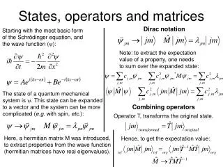
1. States, operators and matrices Dirac notation Starting with the most basic form of the Schrödinger equation, and the wave function (): Note: to extract the expectation value of a property, one needs to sum over the expanded state: The state of a quantum mechanical system is . This state can be expanded to a vector and the system can be more complicated (e.g. with spin, etc.): Combining operators Operator T, transforms the original state. Here, a hermitian matrix M was introduced, to extract properties from the wave function (hermitian matrices have real eigenvalues). Hence, to get the expectation value:

2. Adding spin (1) • Projection is known (m quantum number) • Length of the two spins is known (j1 and j2) • Several possibilities to construct projection by adding the two spins Example: m = jmax - 2 j1 - 2 j2 < j1, j1 - 2 | j2, j2 > < j1, m1 | j2, m2 > = jmax - 2 m

3. Adding spin (1) • Projection is known (m quantum number) • Length of the two spins is known (j1 and j2) • Several possibilities to construct projection by adding the two spins Example: m = jmax - 2 j1 - 1 j2-1 < j1, j1 - 1 | j2, j2 - 1> < j1, m1 | j2, m2 > = jmax - 2 m

4. Adding spin (1) • Projection is known (m quantum number) • Length of the two spins is known (j1 and j2) • Several possibilities to construct projection by adding the two spins Example: m = jmax - 2 j1 j2- 2 <j1, j1 | j2, j2 - 2> < j1, m1 | j2, m2 > = jmax - 2 m

5. Adding spin (2) • Projection is known (m quantum number) • Length of the maximum total spin known jmax = j1 + j2 • Several possibilities to construct projection from different sizes of total spin j j1 j2 | j1 –j2 | ≤ j ≤ j1 + j2 j Note: j1, j2 and j can be interchanged. However, changing the composite state with one of the constituent states is not trivial and requires re-weighting of the constituent states j = j1 + j2 j = j1 + j2 -1 j = j1 + j2 -2 } < j1 + j2, j1 + j2 - 2> < j, m> = jmax - 2 < j1 + j2 - 1, j1 + j2 - 2> m ≥ j m < j, m> = < j, m> = < j1 + j2 - 2, j1 + j2 - 2>

6. Adding spin (3) • Note: - j1 m1 j1 , thus m1 has (2 . j1+1) possible values and m2 (2 . j2 +1). Each combination shows up exactly ones in the second column of the table so the total number of states is (2 . j1+1) (2 . j2 +1). • The third column has the same amount of states as the second column. The quantum number j is a vector addition, thus it will never be lower than |j1 – j2|, which is called jmin. • For m < jmin the amount of states is jmax – jmin + 1 = (j1+j2) – |j1 – j2| + 1 for each m. This situation occurs for - |j1 – j2|  m  |j1 – j2| , thus (2 |j1 – j2| + 1) times. Number of states: (2 |j1 – j2| + 1) . [(j1+j2)-|j1 – j2| + 1] • For m  -jmin and m  jmin the amount of states is jmax  m +1. This results in the following sum: Number of states: • Together these contributions add up to (2 . j1 + 1) (2 . j2 + 1)

7. j = j1 + j2 j = j1 + j2 -1 j = j1 + j2 -2 j1 j2- 2 jmax - 2 m jmax - 2 m Adding spin – Clebsch Gordan Example: m = jmax - 2 e.g. From symmetry relations and ortho-normality, the C coefficients can be calculated. The first few: JM m1,m2

8. Combining spin and boost Lorentz transformations: For: Jackson (section 11.7) calculates the corresponding operator: Extracting rotations: Allowing definition of the canonical state:

9. Intermezzo: rotation properties • The total spin commutes with rotation • However, the projection is affected with a phase. Consider the rotation around the quantization axis • Euler rotations, convention: z y’ z’’ Advantage: quantization axis used twice for rotation • Rotations are unitary operators. The rotation around y’ includes a transformation of the previous rotation. • This results in: i.e. Rotations can all be carried out in same coordinate system when order is inverted.

10. Intermezzo: the rotation matrix Summary of the result from the previous page • Euler z y z convention makes left and right term easy • The expression for djm´m is complicated, but is used mainly for the deduction of symmetry relations: Note 2: Since rotations are hermitic, the conjugate matrix is: Djm’m(-,-,-)=Dj*mm’() Note 1: Inverse rotation is accomplished by performing the rotations through negative angles in opposite order: ( Djm’m(,,) )-1 = Djm’m(-,-,-) Note 3: Combination of all this gives: Dj*m’m()=(-)m’-mDj-m’,-m()

11. Rotations, boosts and spin Describing the rotation of a canonical state: Remember: i.e. rotation of a canonical state rotates the boost and affects the spin state in the same way as it would in the `particle at rest’ state.

12. Helicity The helicity state is defined with: Note: Compared to the same operations on the spin state: Hence: Note that the helicity state does not change with rotations: In other words: helicity () is the spin component (m) along the direction of the momentum. Note that the helicity state does not change with boosts (as long as the direction is not reversed):

13. Discrete symmetries Parity Charge conjugation Dirac: particle Conjugating+transposing gives: Commutation relations: C is the matrix doing the transformation: Mirror analogy Resulting in: Left-handed Left-handed antiparticle e.g.

14. c b Vcb* W+ Vcs Vcb* s b c c W+ Vcs c s Time reversal e.g. Note that time reversal changes t in –t and input states in output states (in other words: < bra | to | ket > ). Another way to show this: i.e. the transformed state does not obey the description of motion of the Hamiltonian, it needs an extra ‘–’ sign. The solution is to make time reversal anti-unitary: Note: this can also be shown with the commutation relation:

15. Time reversal continued Next, the the time reversal operator is split in a unitary part and a complex conjugation. The m states consist of real numbers, i.e. projections. Hence a time reversed expectation value can be described with: Calculating the expectation value of operator Â: And combining with the time reversal operator: Since a second time reversal should restore the original equation: Hermitic

16. Time reversal and spin From the commutation relation: Consistent with: And: The equation: holds if:

17. Time reversal and spin continued Time reversal of a canonical state: Time reversal of a helicity state: Hence: Should give:

18. Parity and spin The parity operation on a canonical state: The parity operation on a helicity state: Hence: Should give: but: Note: Since helicity states include rotational properties:

19. Note: M = m1 + m2 Composite states Bs ground state: b-quark s-quark Bs-meson J/-meson (easy to detect) This ground state can decay to two vector mesons: Isospin = 0 Spin = 1 Parity = - (C-parity = -) c-quark c-quark W+ Bs-meson -meson Isospin = 0 Spin = 1 Parity = - (C-parity = -) b-quark s-quark Isospin = 0 Spin = 0 Parity = - s-quark s-quark

20.  Two body decay properties Spin states of Bs, J/ and : Not the complete story… Consider momentum in two particle decay (Bs rest frame): = Normalization Hence: Remember: Still no complete story… Consider angular momentum: With: Total spin Angular momentum Missing: Formalism that describes angular momentum and Yml states.

21. Rotation with angular momentum Split up the Yml state, to match with new rotation: i.e. the transformation is a product of the rotation of two rest states:

22. Angular momentum and spin We can also express them as states with a sum of angular momentum and spin: Note: MJ = m + MS Note: MS = m1 + m2 Since: (see 1 page back) And: The state can be rotated with: Note that (as expected) the sum of angular momentum and spin (J) is not affected by the rotation, neither are the angular momentum (l) and the total spin (S). This result is the equivalent of the non-relativistic L-S coupling.

23. Two body decay and helicity (1) As with spin, we need to consider momentum in the helicity state: Angles are zero. Particles are boosted back to back along the positive and negative Z-axis The link with previous page is provided via the relation between canonical and helicity states: Single state normalization. Rest mass: w Momentum: p MS = m1 + m2  = 1 - 2 Why?

24. Two body decay and helicity (2) Expressing states with the sum of angular momentum and spin in helicity states: Intermezzo, check… NJ Normalization (later, easier the other way around)

25. Two body decay and helicity (3) Check the transformation properties for rotations: Transforms as it should… Remember: i.e. Mj transforms, but 1 and 2 do not.

26. Canonical versus helicity states (2 pages back) (3 pages back) Combine (4 pages back) Normalization

27. Decay amplitudes Remember: The transition amplitude to a helicity state is calculated with the matrix element: Momentum of decay products: p Resonance rest mass: w And: Complete set With: Check… Hence: Helicity amplitude

28. Helicity amplitude Remember: Switch to canonical states: And: Complete set Partial wave amplitude: als Canonical states

29. Vcb* J/ c Vcs s b c s b c s Bs0 W+  s s Bs0 Bs0 → J/ , tree level J/ s Vcs Bs0 W W- W  s b c Vcb* Oscillation Decay

30. The basics Schrödinger No mixing, just 2 states Particle and anti-particle: Eigen states of the Hamiltonian: en Time evolution of eigen states

31. The basics Mixing: Hermitic: Note: to obtain properties with real values, the matrix needs to be Hermitic.

32. The basics The matrix equation is 0 if: Eigen-states:

33. The basics Eigen-states: Note: The Hamiltonian describes the quantum mechanical system. Only for the eigen-states of the Hamiltonian Mass and Decay time have meaning Note 1: No particle and anti-particle. Two different masses and decay times Note 2: What is the meaning of time (t) at this point. This is a composite system, one particle contains two states. The time is calculated in the restframe of the particle… On the next slide it becomes obvious.

34. The basics Note: So time (t) is just the decay time of the measured particle.