Infiltration
Infiltration. Purpose of infiltration models Irrigation planning Drainage calculations Hydrological models Soil erosion models. Measurement double ring method - gives values which are too high for soil erosion studies, so best use

Infiltration
E N D
Presentation Transcript
Purpose of infiltration models • Irrigation planning • Drainage calculations • Hydrological models • Soil erosion models
Measurement • double ring method - gives values which are too high for soil erosion studies, so best use rainfall simulators for this purpose - but method is fine for surface irrigation design • rainfall simulator (best for sprinkler irrigation design and hydrological modelling)
Modeling Some workers have used texture, bulk density (e.g.) to predict infiltration but reality is complicated by e.g. roots, fauna, tillage system, etc. so be cautious with equations
Philip’s equation (1957) Used Darcy-Richard equation and continuity equation to show that accumulated infiltration: I is the accumulated infiltration S is called the sorptivity (related to rate at which soil absorbs water) measured by horizontal infiltration A is related to saturated hydraulic conductivity (rate at which water passes through soil). At very long times, A approaches the hydraulic conductivity.
The infiltration rate, dI/dt at some time, t is given by: To solve equation for accumulated I, tabulate t and t1/2 for each I, then treat as independent variables, x1 and x2 so I = Sx1 + Ax2 This can be solved in Minitab (not Excel) under “Stats - regression” (untick intercept box)
Kostiakov (1932) I = c t a dI/dt = i = c a t a-1 Infiltration rate declines with time soa - lis always negative. Thus, ais always less than 1. This means that for large times, the rate is 0, which is not true either experimentally or physically. For example, if a = 0.5, thena-1 = - 0.5 so infiltration rate = constant x1/ t 0.5. When t = 100,1/t0.5 = 0.1. When t=10000,1/t 0.5 = 0.01, and so on
To find a and c, tabulate logarithms of I and t in Excel. If y = log I and x = log t, and k=log c then y = k + ax so plot y against x and plot the curves and “Add Trendline” using the “include equation” option. The slope of the line is a and the intercept is k from which you can calculate c
Parameters for Kostiakov's and Philip's equations for a variety of soils [I in inches, t in minutes]
Distribution of Kostiakov’s parameters for some soil textural groups (I in mm, t in minutes)
Green-Ampt (1911) Based on analysis of the physics but not as thorough as Philip’s :- i = ic + b/I ic is the asymptotic infiltration rate at t = and I is very large. However, when t=0, and therefore I=0, the equation predicts infiltration rate is infinite which is also not correct. The equation can also be expressed as: I = ic - B/t where B = gradient of infiltration curve against 1/time.
To solve, plot I against 1/t and find the slope and the intercept
Horton (1940) • i = ic + (i0 - ic)e -kt • i = i0 at t = 0; • ic is the “final” infiltration rate • k is a measure of the rate at which infiltration approaches final value; • mathematically consistent but cumbersome to use in practice because of 3 variables and the exponential curve
There could be more elegent solutions but the following is a workable method. Calculate i over each time increment. The time that applies will be midway between the observed times for accumulated infiltration. Plot i against these values for time and use Excel to Add Trendline using a degree 5 polynomial remembering to use the “include equation” option. Assume that i0 is the intercept given by this polynomial. The value for ic must be less than the final observed value. Set up a range of possible values from 0.5 x final value to 1.0 x final value.
By taking natural logarithms of each side of the equation, it can be shown that ln (i-ic) = ln (i0 - ic) - kt Rearranging this, ln (i0 - ic) - ln (i-ic) = kt You can now tabulate the left hand side against time. Use Excel to calculate the Correlation Coefficient for column corresponding to each different value of ic. The best value for ic will be the one with the highest correlation coefficient. Otherwise use programmes like SAS
Holtan (1961) • i = ic + a (M - I)n • M is the water storage capacity (total porosity antecedent water content), above first impeding stratum. • No meaning if no impeding layer • Only holds for 0 < I < M so I > M must set • i = ic
To solve, again ic must be less than the final observed infiltration rate so try values in the range between from 0.5 x final rate and 1.0 x final rate. For each value of ic plot log (i-ic) against log (M-I). This should be a straight line. Use the correlation coefficient for the columns corresponding to each value of ic to determine the best line. The slope will be n and the intercept will be log a.
Typical infiltration curves • After 5 hours, • high intake-rate soils may have infiltration rate of 60 to 100 mm h-1 • medium intake-rate soils may have infiltration rate of 25 mm h-1 • low intake-rate soils may have infiltration rate of 1 to 4 mm h-1 • Amounts of infiltration may be: • 200 mm after 2 hrs for high intake-rate; • 200 mm after 6 hrs for moderate intake-rate; • 200 mm after 25 hrs for a low intake-rate No universally recognised classification system.
Classification of infiltration curves The following curves are suggested as the basis of a possible system:
These are based on the following values for Philips’ A & S I=At+St0.5 where t in mins, I in mm
Curve 1 or faster: extremely rapid Curves 1 to 2: very rapid Curves 2 to 3: rapid Curves 3 to 4: moderately rapid Curves 4 to 5: moderate Curves 5 to 6: moderately slow Curves 6 to 7: slow Curves 7 to 8: very slow Curve 8 or slower: extremely slow
The slope of the preceding accumulated infiltration curves look like this
It should be noted that the distribution of infiltration rates is log-normal and skewed. The results of one experiment at a single site are shown in the following diagram.
SCS Curve Number concept • Rainfall (P) ends up as either : • total runoff (Q), • retention (G), • initial abstraction (Ia). Ia is the abstraction corresponding to losses from a combination of early infiltration (before runoff), interception (on vegetation) and surface retention (puddles).
The model is based on the observation that ratio of actual infiltration (G) to the maximum potential infiltration (S) is equal to the ratio of the actual runoff (Q) to the maximum potential runoff (P – Ia). It is assumed that both ratios are zero at time equal zero and approach one for time equal infinity for an infinite rain event. Actual infiltration is given by rainfall minus the initial abstraction minus the runoff, i.e. G = (P - Ia) -Q
It was also found that in many situations Ia was approximately equal to 0.2S. This has been used in the preparation of graphs and tables in most text books. (If other relationships were used in the following equations, the graphs and the tables in the handouts would need to be recalculated.) If Ia = 0.2 S, the previous equation becomes :-
Values of S were worked out for different catchment conditions. S is usually expressed as a “curve number”, N such that When S is 0, N is 100 -> 100% runoff Lowest N in practice is about 6.
Some problems with infiltration and soil water flow models (based on Youngs, 1995) • Effect of soil air • trapped, air-filled pores • compression of air in front of wetting front when there is no escape • viscosity of air is not negligible so may be effect even when there is an escape route • Soil heterogeneity • spatial and vertical heterogeneity • random but governed by laws of probability • fingering/instability when less permeable > more permeable
Soil aggregation • macropores and micropores, • domain theory • bypass flow • natural processes / cultivation effects • aggregates may become isolated with little moisture transfer • entrapped air in aggregates may become compressed
Soil instability Structural breakdown and shrinking/swelling cause time dependent soil physical properties
Non-Darcian flow • Soil water may not behave as classical fluid, especially where there are electrically charged soil colloids; • Reynolds's number is used to predict type of flow (turbulent, laminar). R is a function of dimensions of flow channel/pipe, viscosity, velocity. Darcy's law fails at R>1, which it is during infiltration; • Swelling / shrinking means that the frame of reference is moving! Geometry (shape) of structure is not constant swelling is not uniform in all directions
Clay particles in suspension also move • In clay soils, part of the overburden is transmitted to the soil water- has to be allowed for in equations, proportion depends on the moisture content
Non-isothermal flow • Theory assumes isothermal conditions but there are thermal gradients near the surface and the heat of wetting generated at the wetting front. • Hysteresis • Hysteresis can be incorporated but diffusivity • becomes discontinuous which makes analysis more • difficult.
Anisotropy • Solutions assume isotropic media - not true in real soils • Conductivity in horizontal direction may be different (usually slower) from the vertical direction • Anisotropic because of cracks, worm holes, etc.
Effects of structure Structure has a great effect on infiltration. For loam, range can be from 1.5 mm h-1 for massive structure to 150 mm h-1.for well structured. Improved structure e.g. by roots and infiltration will increase, runoff will decrease, erosion will decrease.
Effect of vegetation Vegetation causes the soil to be more "open" and increases infiltration. One relationship is :- Kveg is the conductivity with vegetation, Ksatis the conductivity without vegetation ais the fraction of ground covered with vegetation at the base.
Alteration For water harvesting, sometimes infiltration needs to be reduced (covered in 556 - Water Harvesting and Use of Chemicals)