Future of Web-Based Knowledge Acquisition and Self-Innovation
610 likes | 825 Vues
Explore the benefits of web-based learning, knowledge acquisition, and self-improvement techniques using advanced technology tools. Enhance lifelong learning skills with transparent grading and self-management. Develop a personalized system for promoting and sharing activities anytime, anywhere.

Future of Web-Based Knowledge Acquisition and Self-Innovation
E N D
Presentation Transcript
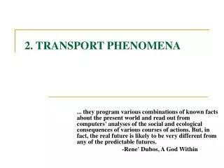
2. TRANSPORT PHENOMENA ... they program various combinations of known facts about the present world and read out from computers' analyses of the social and ecological consequences of various courses of actions. But, in fact, the real future is likely to be very different from any of the predictable futures. -Rene' Dubos, A God Within
웹 기반 지식 정보 획득 및 자기 혁신 기법 • 웹 기반 기술을 활용함으로서 자기 능력을 최대한 개발 • 가상강좌의 효과를 최대화하여 수강생의 지식 습득을 최대화 • 모든 수업 내용은 시공간에 제약없이 웹 상에서 습득 • 모든 수업 내용은 MP3 파일로 제작하여 수강생이 항상 습득 가능함. • 수업에 관계된 모든 내용은 비디오 파일로 저장되어야 함 • 수강생은 면대면 강의에 필히 참여하여야 함 • 면대면 강의 혹은 실습시간은 수강생이 진행 : 기존의 강의 내용 및 숙제 등을 본인의 웹 서버에 구축하여 발표 • 면대면 강의나 기타 수강생의 모든 활동 내용은 비디오 파일로 녹화되어 웹 상에서 제공됨으로서 투명한 성적관리와 수강생의 자기 관리 및 경쟁심 유도 • 본 수업뿐만이 아니라 수강생의 평생 지식 습득 기술 획득 • 자신과 관련된 모든 활동을 녹화하고 웹 상에서 관리 함으로서 시공간에 제약없는 자기관리 가능 • 본인의 홍보를 위한 시스템으로 활용 : 시공간에 제약없는 정보통신 가능 : 본인의 모든 활동을 필요한 경우 홍보 및 공유 • 모든 수강생은 마이크가 내장된 웹 캠을 구입하여 자기 관리 시스템 구축 • 정보 통신 기술의 발전으로 휴대폰에서 이러한 시스템이 작동될 것임.
Contents • 2.1 Introduction: 3 motion processes (advective, dispersive, and sediment transport) • 2.2 Advection • 2.3 Diffusion/Dispersion: molecular diffusion, turbulent diffusion, dispersion 2.3.1 Analogies Between Mass, Momentum, and Heat Transfer 2.3.2 Fick’s Second Law 2.3.3 Advection-Dispersion Equation 2.3.4 Solutions to Advection-Dispersion Equation and Tracer Experiments 2.3.5 Longitudinal Dispersion Coefficient in Rivers 2.3.6 Lateral Dispersion Coefficient in Rivers 2.3.7 Vertical Dispersion Coefficient in Rivers 2.3.8 Vertical Eddy Diffusivity in Lakes • 2.4 Comparmelization 2.4.1 Choosing a Transport Model 2.4.2 Compartmentalization and Box Models • 2.5 Sediment Transport 2.5.1 Partitioning 2.5.2 Suspended Load 2.5.3 Bed Load 2.5.4 Sedimentation 2.5.5 Scour and Resuspension 2.5.6 Desorption/Diffusion • 2.6 Lake Dispersion Calculations 2.6.1 McEwen's Method 2.6.2 Heat Budget Method • 2.7 Simple Transport Models 2.7.1 Completely Mixed Systems (CSTR) 2.7.2 Plug-Flow Systems 2.7.3 Advective-Dispersive Systems 2.7.4 Closure • Problems
2.1 INTRODUCTION • Rate of a chemical's transport in the aquatic environment - equally important process as the reactions that a chemical may undergo • Three processes of mass transport in aquatic ecosystems: • transport by the current of the water (advection) • transport due to mixing within the water body (dispersion) • transport of sediment particles within the water column and between the water and the bed (benthos) • Toxic chemicals exist in a dissolved phase and a sorbed phase. • Dissolved substances are transported by water movement with little or no "slip" relative to the water. • Chemicals that are sorbed to colloidal material or fine suspended solids are essentially entrained in the current, but they may undergo additional transport processes such as sedimentation and deposition or scour and resuspension. • In order to determine the fate of toxic organic substances, we must know both the water movement and suspended sediment movement. • The transport of toxic chemicals in water: • advection (refers to movement of dissolved or very fine particulate material at the current velocity in any of three directions • dispersion (refers to the process by which these substances are mixed within the water column; can also occur in free directions)
Figure 2.1 Schematic of transport processes: (1) advection, movement of chemical entrained in current velocity; (2) turbulent diffusion, spread of chemical due to eddy fluctuations; and (3) dispersion, spread of chemical due to eddy fluctuations in a macroscopic velocity gradient field.
Three processes contribute to mixing (dispersion): Molecular diffusion • the mixing of dissolved chemicals due to the random walk of molecules within the fluid, caused by kinetic energies of molecular vibrational, rotational, and translational motion • corresponds to an increase in entropy whereby dissolved substances move from regions of high concentration to region (of low concentration according to Fick's laws of diffusion) • generally not an important process in the transport of dissolved substances in natural waters except relating to transport through thin and stagnant films at the air-water interface or transport through sediment pore water) Turbulent diffusion • refers to mixing of dissolved and fine particulate substances caused by microscale turbulence • an adjective process at the microscale level caused by eddy fluctuations in turbulent shear flow • Shear forces within the body of water are sufficient to cause this form of mixing • several orders of magnitude larger than molecular diffusion • contributing factor to dispersion. • can occur in all three directions but is usually anisotropic (i.e., there exist preferential directions for turbulent mixing due to the direction and magnitude of shear stresses).
Dispersion • The interaction of turbulent diffusion with velocity gradients caused by shear farces in the water body causes a still greater degree of mixing known as dispersion • Transport of toxic substances in streams and rivers is predominantly by advection, but transport in lakes and estuaries is often dispersion-controlled. • Velocity gradients • caused by shear forces at the boundaries of the water body, such as vertical profiles due to wind shear at the air-water interface, and vertical and lateral profiles due to shear stresses at the sediment-water and bank-water interfaces (Figure 2.2). • due to channel morphology and sinuosity or meandering of streams. Secondary currents develop in stream and river channels that account for a great deal of mixing.
Figure 2.2 Schematics of velocity gradients created by shear stresses at the air-water, bed-water, and bank-water interfaces Figure 2.3 Secondary current in a stream responsible for lateral and longitudinal dispersion.
2.2 ADVECTION • For a chemical traveling in a stream or a river, advective transport is the product of the volumetric flow rate and the mean concentration (that is, the amount of a substance moving in the water). Flux: • Mass inside the control volume, at any instant, may be written as volume times concentration – V*C • The change in mass in control volume with respect to time due to advection may be written as: △mass = (Mass inflow rate - Mass outflow rate)△time Ca is the concentration entering the incremental control volume, Cbis the concentration leaving the control volume. • Differential equation describing advection of mass under time-varying conditions . • Total mass that has passed a point in a given amount of time
Example 2.1 Advective Transport of Pesticide in a River Calculate the average mass flux (in kg d-1) of the pesticide alachlor passing a point in a river draining a large agricultural basin. The mean concentration of of pesticide is 1.07 μgL-1, and the mean flow is 50 m3s-1. Is this an accurate estimate of the total mass passing this point in a year, considering high runoff events? • Average mass discharge (kgd-1) with respect to flowrateis Using the annual average concentration and annual average flowrate does not give the total annual mass discharge passing a point because flowrate and concentration are positively correlated. High flows create high pesticide concentrations due to agricultural runoff. The mass discharge rate calculated above underestimates the total average mass discharge rate for the year. Use the following equation to estimate the total mass passing a point during the year. The average mass discharge, , is equal to the average flowrate timed average concentration, , plus the average mass fluctuation, .
2.3 DIFFUSION / DISPERSION • In 1855, Fick published his first law of diffusion based on movement of chemicals through fluids under quiescent conditions. • the analogy to Fourier's law of heat conduction • molecular diffusion results from the translational, vibrational, and rotational movement of molecules through a fluid, in this case water. • energetically it is a spontaneous reaction, and it results in an increase in entropy (tendency toward the random state) Jm is the mass flux rate due to molecular diffusions, MT-1; A is the cross-sectional area, L2;dC/dx is the concentration gradient, ML-3L-1; D is the molecular diffusion coefficient, L2T-1; F is the areal mass flux rate, ML-2 T-1
Figure 2.5 Diffusive transport from point a to point b. At the beginning of the experiment (t = 0) all of the chemical is dissolved in the beaker on the left-hand side. When the experiment begins, mass moves from areas of high concentration to areas of low concentration according to Fick's laws of diffusion until equilibrium is established
Example 2.2 Molecular Diffusion of a Chemical • Calculate the mass flux rate in mg d-1 for a chemical diffusing between two beakers, such as shown in Figure 2.5. Assume the chemical is diffusing through a 10-cm distance with a concentration gradient of -1 mg L-1 cm-1 • This is an incredibly slow rate of mass transfer considering that it would take 1 year to transport 1 mg of chemical if the concentration gradient was held constant over time. (The experiment in Figure 2.5 actually shows a nonsteady state condition.)
Example 2.3 Molecular Diffusion Through a Thin Film • The molecular diffusivity of caffeine (C9H8O) in water is 0.63×10⁻⁵cm2s-1. For a 1.0mg L-1 solution, calculate the mass flux in mg/s through an intestinal membrane (0.1-m2 area) with a liquid film approximately 60μm thick. How long would it take 1 mg of caffeine to move through 0.1 m2 of intestine, assuming the above flux rate? (Note: We assume transport through the film is the rate-limiting step in transport and metabolism.) (assume zero caffeine inside intestine)
2.3.1. Analogies Between Mass, Momentum, and Heat Transfer • 1877, Boussinesq: first proposed that turbulent momentum transport is analogous to viscous momentum transfer in laminar flow. • 1894, Reynolds: the same suggestion, he showed clearly the critical dimensionless number (Re = 2300) necessary to change from laminar flow to turbulent flow in pipes Re is Reynolds Number, u is mean velocity(LT-1), d is pipe diameter (L), ν is kinematic viscosity(L2T-1) • Figure 2.6: mass, heat, and momentum transport can occur simultaneously and they are all analogous. The flux rate per unit area is a gradient driving force times a proportionality constant for the turbulent flow field (ε). • Table 2.1 gives the definition fur the "proportionality" constants among mass, heat, and momentum transport processes under laminar or turbulent flow conditions . • The dimensionless ratio between thermal diffusivity and mass diffusion coefficient is termed the Lewis number. Its value determines the extent of analogy between heat and mass transfer; under turbulent conditions, it can vary from 1.0. • Dimensionless numbers relating kinematic viscosity to mass diffusion coefficients (the Schmidt number) and kinematic viscosity to thermal diffusivity (Prandtl number) may also vary from 1.0 in simultaneous heat mass, and momentum transfer.
Figure 2.6 Analogous and simultaneous transfer of momentum, mass, and heat transfer in a turbulent river. (a) Shear forces at the sediment-water interface create a vertical velocity field that transfers momentum downward (b) A contaminated sediment transfers mass to the water column by vertical turbulent diffusion (c) Summer stratification of the river creates a vertical heat flux downward
Proportionality constants for dispersion, turbulent diffusion, and molecular diffusion can differ by orders of magnitude for different processes , but they all are expressed in the same units and are used in a "Ficks law" type of equation. The driving farce in each case is the concentration gradient, dC/dx. Dispersion coefficients are much greater than eddy diffusivities which are, in turn, much larger than molecular diffusion coefficients. • Jt is the mass flux rate due to turbulent diffusion , εm is the turbulent diffusion coefficient (or turbulent diffusivity), Jd is marts flux rate due to dispersion, E is the dispersion coefficient. • There is an initial period of mixing, during which the Fickian analogy far dispersion is not valid. This is due to the scale of turbulent diffusion and differential advection filling a fully developed flow regime. After the initial release of a slug of tracer, it takes some time for conditions to develop that can be described by the Fickian analogy.
2.3.2 Fick’s Second Law • Fick's second law of diffusion follows from the first law of diffusion under non-steady state as follows: • The above quation is a second-order partial differential equation so it requires two boundary conditions (one for each order) and one initial condition in order to solve. Solutions to this equation are many and varied - there is a different solution for each set of boundary and initial conditions that may be posed • Integrating the above equation may be accomplished by separation of variables, Laplace Transformation, Boltzmann Transformation, or by trial and error methods, depending on the boundary conditions posed.
Example 2.4 Diffusion from a Contaminated Sediment (Gauss solution for diffusion equation) • Solve Fick's second law of diffusion. The problem is for vertical eddy diffusion from a planar source (a contaminated lake sediment) to the overlying water column. IC and BC’s (for a semi-infinite water column: early stages of diffusion) are as folows: • Seek the solution through trial-and-error solution for an instantaneous planar source. A is an arbitrary constant • Take the partial derivative of the above equation with respect to time and the second partial derivative w.r.t.x. Use integral tables far "derivative of a product" and eu. • The partial derivative w.r.t. time is:
The second derivative with respect to vertical distance, x, is • This is the same result as for ∂C/∂t above, which proves that the solution will work. Now it is necessary to solve for the arbitrary constant, A, in terms of the mass diffusing, M: • Using the definite integral identity below, the exponent is of the form : • By the principle of reflection at the x = 0 plane:
Under the influence of larger and larger mixing scales, the eddys that influence a given solute molecule increase the proportionality of mixing. Prandtl in 1925 introduced the concept of mixing length, a measure of the average distance a fluid element would stray from the mean streamline. • The probability of a chemical solute being entrained by ever-larger eddies increases with time and the scale of the problem. It was proposed by Richardson that horizontal eddy diffusivities in the ocean increase with the length of the solute plume to the four-thirds power. • εm - the mass eddy diffusivity, cm2 s-1, L is the length scale of the plume in cm, 0.01 is a proportionality constant for units in the cgs system. Under these conditions the diffusion equation becomes • Figure 2.7 shows a log-log representation of equation for mass eddy diffusivity over some seven orders of magnitude in length scale .
Figure 2.7 Thermal stratification in a lake and the assumption of mixing between two compartments.
2.3.3 Advection-Dispersion Equation • The basic equation describing advection and dispersion of dissolved matter is based on the principle of conservation of mass and Fick's law. • (Homework) Derive Mass Transport Eq’n from Mass Balance • C is concentration (ML-3), t is time (T), ui is average velocity in the ith direction (LT-1), xi is distance in the i-th direction (L), R is reaction transformation rate (ML-3T-1), Ei is the diffusion coefficient in the i-th direction. • Expressing the equation in Cartesian coordinates results in
Under nonsteady flow conditions, the velocity in the longitudinal direction can vary in space and time. For a one-dimensional river, • To solve the above equation analytically would require exact (and simple) functional relationships for A, Q, and E, but in practice the nonsteady transport equation is solved numerically, and it is coupled to numerical solutions of open-channel flow such as the St.Venant equations: : 개수로 유동의 continuity equation : equation of motion : friction term • b is width at water level (L), f is Darcy-Weisbach friction factor, g is gravitational acceleration constant (L2T-1), P is wetted perimeter (L), qi is lateral inflow per unit length of river (L2T-1), Q is flowrate (discharge) (L3T-1), z is absolute elevation of water level above datum (L)
If the velocity and cross-sectional area of the river are nearly constant with respect to time (steady flow) but changing in space, mass stransport equation can be simplified to • The simplest form of the advection-dispersion equation for one-dimensional rivers is given by the below equation when A, Q, and E are all constant with respect to time and distance. • The above equation may not be exact for many model applications where river velocity and dispersion coefficient vary with longitudinal distance, but it can be useful if applied in segments of the river in which ux and Ex are constant. The river can be segmented into pieces of relatively constant flow and morphometry, and a new segment can be initiated at each point source discharge of the chemical of interest.
2.3.4 Solutions to Advection-Dispersion Equation and Tracer Experiments • Tracers : dyes (e.g., Rhodamine WT), salts, stable isotopes • To determine the transport characteristics of a natural water body • The advection and dispersion of dye (tracer) in a 3-D velocity field (variable dispersion in each direction) has been solved (zero-reaction) • If the dye has been well mixed with depth, the 3-D equation can often be released to a two-dimensional problem
2.3.5 Longitudinal Dispersion Coefficient in Rivers • Liu used the work of Fischerto develop an expression for the longitudinal dispersion coefficient in rivers and streams (Ex, which has units of length squared per time): • β – 0.5 U*/ux; D – mean depth, L; B – mean width, L; U* - bed shear velocity, LT-1; ux – mean stream velocity, LT-1; A – cross-sectional area, L2; QB – river discharge, L3T-1 • βdoes not depend on stream morphometry but on the dimensionless bottom roughness. • Based on existing data for Ex in streams, the value of Ex can be predicted to within a factor of 6 by the above equation. • The bed shear velocity is related empirically to the bed friction factor and mean stream velocity: τ0 is bed shear stress, ML-1T2; f – Darcy-Weisbach friction factor ≈ 0.02 for natural, fully turbulent flow; ρ – density of water, ML-3
2.3.6 Lateral Dispersion Coefficient in Rivers • Φ = 0.23 (experimentally obtained in long, wide laboratory flumes) • Sayre and Chang: Φ = 0.17 in a straight laboratory flume. • Yotsukura, Cobb, Yotsukura, Sayre: for natural streams and irrigation canals Φ varying from 0.22 to 0.65, with most values being near 0.3. • Other: Φ in the range from 0.17 to 0.72. • The higher values for are all for very fast rivers and bends. • The conclusions drawn are: (1) the form of the above equation is correct, but may vary (2) application of Fickian theory to lateral dispersion is correct as long as there are no appreciable lateral currents in the stream. • Elder’s lateral dispersion coefficient Ey
2.3.7 Vertical Dispersion Coefficient in Rivers • Very little experimental work has been done on the vertical dispersion coefficient, Ez. Jobson and Sayre • z is vertical distance, k is the von Karman coefficient, which is shown experimentally to be approximately = 0.4
2.3.8 Vertical Eddy Diffusivity in Lakes • Vertical mixing in lakes is not mechanistically the same as that in rivers. . • The term "eddy diffusivity" is often used to describe the turbulent diffusion coefficient for dissolved substances in lakes. • Chemical and thermal stratification serve to limit vertical mixing in lakes, and the eddy diffusivity is usually observed to be a minimum at the thermocline. • Many authors have correlated the vertical eddy diffusivity in stratified lakes to the mean depth, the hypolimnion depth, and the stability frequency. • Mortimer’s vertical diffusion coefficient • Vertical eddy diffusivities can be calculated from temperature data by solving the vertical heat balance or by the simplified estimations of Edinger and Geyer . • Schnoor and Fruh demonstrated that the mineralization and release of dissolved substances from anaerobic sediment can be used to calculate average hypolimnetic eddy diffusivities. This approach avoids the problem of assuming that heat (temperature) and mass (dissolved substances) will mix with the same rate constant, that is, that the eddy diffusivity must equal the eddy conductivity. • A summary of dispersion coefficients and their order of magnitude appears in the table below.
A summary of dispersion coefficients and their order of magnitude • Vertical dispersion coefficients in lakes have most commonly been determined by the heat budget method or by McEwen's method; radio-chemical methods also have been used.
2.4 COMPARTMENTALIZATION2.4.1 Choosing a Transport Model • Relative importance of advection compared to dispersion can be estimated with the Peclet number. • Pe >> 1.0 advection predominates ; Pe << 1.0 dispersion predominates • If there is a significant transformation rate, the reaction number can be helpful: • K is the first-order reaction rate constant (T-1). 2.4.2 Compartmentalization and Box Models • Compartmentalization refers to the segmentation of model ecosystems into various "completely mixed" boxes of known volume and interchange. • Interchange between compartments is simulated via bulk dispersion or equal counterflows between compartments. • Assumption of complete mixing reduces the set of partial differential equations (in time and space) to one of ordinary differential equations (in time only). • ODE for compartmentalization is as follows.
The above equation can be rewritten in terms of bulk dispersion coefficients • E’ is bulk dispersion coefficient (L2T-1), Aj,k is interfacial area between compartments j and k (L2), lj,k is distance between midpoints of compartments(L). • There is one mass balance equation [such as the above one] for each of the j compartments. This set of ordinary differential equations is solved simultaneously by numerical computer methods . • 호수의 경우 분산계수는 추적제 실험의 결과치를 이용하게 되는 데 전체 연립방정식의 해의 역산으로부터 평가되기때문에 상당히 큰 분산계수값을 가지게 된다. • 하천과 빠르게 흐르는 강에서는 종방향으로는 분산이 존재하지 않으며 해를 구하기 위해서 인위적인 분산계수를 도입한다.
One approach: set the artificial dispersion coefficient equal to the measured or estimated dispersion coefficient from the above equation. • A better approach is to adjust the time step to minimize Ex while preserving stability (특성화or particle tracking method): • One method of estimating the artificial or numerical dispersion of such a compartmentalized model for an explicit upwind differencing method is: • Lakes, reservoirs, and embayments may require a number of compartments if some spatial detailis needed, such as concentration profiles. These compartments should be chosen to relate to the physical and chemical realities of the prototype. E.g., a logical choice for a stratified lake is to have two compartments: an epilimnion and a hypolimnion (figure 2.7). Mixing between compartments can be accomplished by interchanging flows: (J is net mass flux from epilimnion to hypolimnion due to vertical mixing , Qex is exchange flow .
2.5 SEDIMENT TRANSPORT2.5.1 Partitioning • A chemical is partitioned into a dissolved and particulate adsorbed phase based on its sediment-to-water partition coefficient, Kp. The dimensionless ratio of the dissolved to the particulate concentration is the product of the partition coefficient and the concentration of suspended solids, assuming local equilibrium (분배계수에 의해 총부유고형물중 일부는 입자상물질로 일부는 용존물질로 분배됨.) • Cp is particulate chemical concentration(μg L-1), C is dissolved chemical concentration, Kp is sediment/water partition coefficient(L kg-1), M is suspended solids concentration(kg L-1), CT is total concentration. • Bed sediment concentration can be calculated using conccentration of suspended solids in the water and porosity of bed sediment, i.e., Mb=M/n
2.5.2 Suspended Load • The suspended load of solids in a river or stream : flowrate times the concentration of suspended solids (e.g., kg/d or tons /d); the mean load is greatly affected by peak flows. Peak flows cause large inputs of allochthonous material from erosion and runoff as well as increases in scour and resuspension of bed and bank sediment. The average suspended load is not equal to the average flow times the average concentration, and can be calculated as follows:
2.5.3 Bed Load • Several formulas have been reported to calculate the rate of sediment movement very near the bottom. These equations were developed far rivers and noncohesive sediments, that is, fine-to-coarse sands and gravel. It is important to note that it is not sands, but rather silts and clays, to which most chemicals sort. Therefore these equations are of limited predictive value in environmental chemical modeling. • Generally, bed load transport is a small fraction of total sediment transport (suspended load plus bed load). Figure 2.8 Suspended load and bed load. Bed load is operationally defined as whatever the bed load sampler can measure. Bed load occurs within a few millimeters of the fixed bed.
2.5.3 Sedimentation • Suspended sediment particles and adsorbed chemicals are transported downstream at nearly the mean current velocity. In addition, they are transported vertically downward by their mean sedimentation velocity. . • Generally, silt and clay-size particles settle according to Stokes' law, in proportion to the square of the particle diameter and the difference between sediment and water densities: • W = particle fall velocity, ft s-1 ; ρs= density of sediment particle, 2-2.7 g cm-3; ρw = density of water, 1 g cm-3 ; ds = sediment particle diameter, mm ; μ = absolute viscosity of water, 0.01 poise (g cm-1s-1) at 20oC) • Once a particle reaches the bed, a certain probability exists that it can be scoured from the bed sediment and resuspended. The difference between sedimentation and resuspension represents net sedimentation. Often it is possible to utilize a net sedimentation rate constant in a pollutant fate model to account for both processes. • ks= net sedimentation rate constant, W=mean particle fall velocity, H= mean depth.
2.5.5 Scour and Resuspension • Under steady-state conditions, the sedimentation of suspended sediment must equal the scour and resuspension of sediment. • w = sedimentation velocity, L T-1 ; εs = suspended sediment vertical eddy diffusivity, L2 T-1 ; C = concentration of suspended sediment, M L-3. • Under time-varying conditions, however, the boundary condition at the bed-water interface p = probability that descending particle will "stick" to the bed SD = rate of bed deposition, M L-2 T-1 SR = = rate of bed scour, M L-2 T-1 • Mj = erodibility coefficient, ML-2T-1; τcR = critical bed shear required for resuspension, ML-1T-2; τcD = critical bed shear stress that prevents deposition, ML-1T-2; h = ratio of depth of water to depth of active bed layer
2.5.6 Desorption/Diffusion • In addition to sedimentation and scour/resuspension, an adsorbed chemical can desorb from the bed sediment. Likewise, dissolved chemical can adsorb from the water to the bed. Both pathways can be presented by a diffusion coefficient and a concentration gradient or difference between pore-water and overlying dissolved chemical concentrations. • Sediment mass balances must include terms far advection, sedimentation, scour/resuspension, and possibly vertical dispersion. At the bottom, bed load movement may be included. Processes that affect the fate of dissolved substances include desorption from the bed (or adsorption from the water column), advection, dispersion, and transformation reactions. • Often, it is possible to neglect the kinetics of adsorption and desorption in favor of a local equilibrium assumption. Over the time scales of interest, this may be a good assumption. Bed load is sometimes small relative to wash load movement of absorbed chemicals and can be neglected. Under steady-state conditions, net sedimentation rates are often used to simplify the transport of sedimentation and scour.
2.6 LAKE DISPERISON CALCULATIONS • The steps for calculating vertical dispersion across the thermocline in a lake from temperature data are presented below. • These methods were derived from the heat dispersivity equation, assuming that E does not vary much with depth over the region of interest, particularly the thermocline . • It is assumed that no heat has entered the lower part of the water column by any mechanism other than vertical turbulent transport, E. • The assumption is made that mass transfer through dispersion occurs at the same rate as heat transfer. The analogy is applied by substituting concentration or mass (C) into the equation. • θ is temperature, t is time, E is thermal dispersivity, and z is distance 2.6.1 McEwen's Method • This method of computing lake dispersion is based on fitting an exponential curve to the mean temperature data in the thermocline and hypolimnion. If the data are of a linear or otherwise nonexponential shape, this method is inappropriate
2.6.2 Heat Budget Method • The vertical thermal dispersivity also can be estimated from the total heat entering and leaving the lake. A heat budget results in vertical dispersion coefficients that are a function both of depth and time, E = f(z, t) • The basic equation is based on heat transfer and is formulated similar to a mass balance: • Vj is the volume of the jth slice, (m3); θj is the mean temperature in the jth slice (oC); Qi and Qo are inflows and outflows to slice j, Qvj is the vertical flowrate at the bottom of the jth element, where upward flow is positive, (m3s-1); Ej is the dispersion across the bottom of slice j (cm2s-1), aj is the bottom surface area of slice j (m2); t is time (s), hnet is the net heat flux (cal s-1 cm-3); Δz is the thickness (m) of slice (must be the same for all slices)
The heat flux at the surface equals net heat flux/slice thickness as shown below. • β is the fraction of short-wave radiation absorbed at the surface, hs is short-wave radiative flux, ha is long-wave or atmospheric radiative flux, hb is back radiation, he is evaporative energy flux, and hc is convective energy flux • Below the surface, only short-wave radiation is absorbed. In deeper slices, hj’ an exponential function of depth. The quantity of solar radiation absorbed by the jth element is expressed as • long-wave radiative flux • back radiation • evaporative heat flux at the surface • convective heat flux at the surface
2.7 SIMPLE TRANSPORT MODELS2.7.1 Completely Mixed Systems (CSTR) • The mass balance: • Cin = chemical concentration in inflow, ML-3 ; C = chemical concentration in the lake and in outflow, ML-3 ; Qin = volumetric inflow rate, L3T-1 ; Qout = volumetric outflow rate, L3T-1 ; V = volume of the lake, L3 ; r = reaction rate, ML-3L-1; positive and negative signs indicate formation and decay reactions, respectively
Figure 2.9 Schematic of a completely mixed lake, with inputs and effluent responses.
A response to an accidental spill of chemical into a lake can be formulated using the impulse (or delta) function if the discharge of chemical occurred for a relatively short time period. Simple case: conservative tracer is instantaneously injected into the lake as in impulse input the equation may be reduced to • τis mean hydraulic detention time, V/Q. • If Cin, Qin = Qout = Q are constants, dV/dt = 0, r = -kC , mass balance equation becomes • In the event that a reactive chemical was spilled into the lake: • Response to a continuous load, such as a waste discharge from a municipality or an industry to a lake, is represented by the following equation and its steady-state solution.
Nonsteady-state solution can be obtained as follows (by integrating factor method), 1st-order linear differential equation with general form of • If a number of lakes are present in the series, these water bodies can be analyzed collectively. Figure 2.10 shows a series of lakes that consists of n equal-volume, completely mixed lakes. The approach is based on a mass balance around each lake of the series. Generalizing the mass balance equation from the 1st to nth lake, the following solution is obtained:
Figure 2.10 Schematic of completely mixed lakes in series, and effluent responses with reaction decay.
For an impulse input of conservative tracer the time-variable solution can be obtained in successive order from 1st to nth lake as follows: • In the case that a lake or reactor vessel is segmented into n compartments, the effluent response to an impulse input of nonreactive chemical may be given by the equation below. • τ’ is the detention time of an individual lake (Vtotal/Q), Co is the initial concentration if the impulse input were delivered to the entire vessel (M/Vtotal). • 그림 2.11에서 보여주는 바와 같이 구획수가 클수록 플러그 유동 모형으로 구획수가 작을수록 완전혼합모형으로 진행된다. 호수는 플러그와 확산유동의 특성을 다 가지고 있기 때문에 위의 해는 추적자의 순간 유입에 잘 적용되는 이론적인 구간의 개수에서 적용 가능하다.