Download
1 / 19
190 likes | 287 Vues
Exploring collisions in plasma, ionospheric currents, Coulomb interactions, conductivity in magnetized plasmas, effects of collisions on resistivity, and typical collision parameters in space plasmas.

E N D
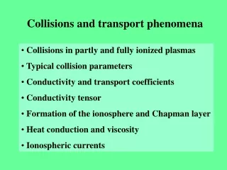
Collisions and transport phenomena • Collisions in partly and fully ionized plasmas • Typical collision parameters • Conductivity and transport coefficients • Conductivity tensor • Formation of the ionosphere and Chapman layer • Heat conduction and viscosity • Ionospheric currents
Collisions Plasmas may be collisional (e.g., fusion plasma) or collisionsless (e.g., solar wind). Space plasmas are usually collisionless. • Ionization state of a plasma: • Partially ionized: Earth‘s ionosphere or Sun‘s photosphere and chromosphere, dusty and cometary plasmas • Fully ionized: Sun‘s corona and solar wind or most of the planetary magnetospheres Partly ionized, then ion-neutral collisions dominate; fully ionized, then Coulomb collisions between charge carriers (electrons and ions) dominate.
Collision frequency and free path The neutral collision frequency, n, i.e. number of collisions per second, is proportional to the number of neutral particles in a column with a cross section of an atom or molecule, nnn, where nn is the density and n= d02 ( 10-20 m2) the atomic cross section, and to the average speed, < > ( 1 km/s), of the charged particle. The mean free path length of a charged particle is given by:
Coulomb collisions I Charged particles interact via the Coulomb force over distances much larger than atomic radii, which enhances the cross section as compared to hard sphere collisions, but leads to a preference of small-angle deflections. Yet the potential is screened, and thus the interaction is cut off at the Debeye length, D. The problem lies in determining the cross section, c. Impact or collision parameter, dc, and scattering angle, c.
Coulomb collisions II The attractive Coulomb force exerted by an ion on an electron of speed ve being at the distance dc is given by: This force is felt by the electron during the fly-by time tc dc/e and thus leads to a momentum change of the size, tc FC, which yields: For large deflection angle, c90o, the momentum change is of the of the order of the original momentum. Inserting this value above leads to an estimate of dc , which is:
Coulomb collisions III The maximum cross section, c = dc2, can then be calculated and one obtaines the electron-ion collision frequency as: Taking the mean thermal speed for ve , which is given by kBTe = 1/2 meve2, yields the expression: The collision frequeny turns out to be proportional to the -3/2 power of the temperature and proportional to the density. A correction factor, ln, still has to be applied to account for small angle deflections, where is the plasma parameter, i.e. the number of particles in the Debye sphere.
Coulomb collisions in the solar wind • N is the number of collisions between Sun and Earth orbit. • Since in fast wind N < 1, Coulomb collisions require kinetic treatment! • Yet, only a few collisions (N 1) remove extreme anisotropies! • Slow wind: N > 5 about 10%, N > 1 about 30-40% of the time.
Plasma resistivity In the presence of collisions we have to add a collision term in the equation of motion. Assume collision partners moving at velocity u. In a steady state collisional friction balances electric acceleration. Assume there is no magnetic field, B = 0. Then we get: Since electrons move with respect to the ions they carry the current density, j = -eneve. Combining this with the above equations yields, E = j, with the resistivity:
Conductivity in a magnetized plasma I In a steady state collisional friction balances the Lorentz force. Assume the ions are at rest, vi = 0. Then we get for the electron bulk velocity: Assume for simplicity that, B=Bez. Then we can solve for the electron bulk velocity and obtain the current density, which can in components be written as: Here we introduced the plasma conductivity (along the field). The current can be expressed in the form of Ohm‘s law in vector notation as: j = E, with the dyadic conductivity tensor .
Conductivity in a magnetized plasma II For a magnetic field in z direction the conductivity tensor reads: When the magnetic field has an arbitrary orientation, the current density can be expressed as: The tensor elements are the Pedersen,D, the Hall,H, and the parallel conductivity. In a weak magnetic field the Hall conductivity is small and the tensor diagonal, i.e. the current is then directed along the electric field.
Dependence of conductivities on frequency ratio |ge| < c, electrons are scattered in the field direction before completing gyration. |ge| > c, electrons complete many gyrocircles before being scattered -> electric drift prevails.
Formation of the ionosphere The ionosphere is the transition layer between the neutral atmosphere and ionized magnetosphere. Solar ultraviolet radiation impinges at angle , is absorbed in the upper atmosphere and creates ionization (also through electron precipitation). I is the flux on top of the layer. The ionosphere is barometrically stratified according to the density law: H is the scale height, defined as, H= kBTn/mng, with g being the gravitational acceleration at height z = 0, where the density is n0.
Diminuation of ultraviolet radiation According to radiative transfer theory, the incident solar radiation is diminished with altitude along the ray path in the atmosphere: Here is the radiation absorption cross section for radiation (photon) of frequency . Solving for the intensity yields: This shows the exponential decrease of the intensity with height, as is schematically plotted by the dashed line in the subsequent figure.
Formation of the Chapman layer The number of electron-ion pairs locally produced by UV ionization, the photoionization rate per unit volume q(z), is proportional to the ionization efficiency, , and absorbed radiation: q(z) = nnI(z). This gives the Chapman production function, quoted and plotted below.
Electron recombination and attachment Recombination, with coefficient r, and electron attachment, r, are the two major loss processes of electrons in the ionosphere. In equilibrium quasi-neutrality applies: ne = ni Then the continuity equation for ne reads:
Transport coefficients: Heat conduction and viscosity Electrons in a collison-dominated plasma can carry heat in the direction of the temperature gradient, Fourier‘s law: Qe = - e Te e = 5nekB2Te/(2mec ) Ions in a collison-dominated plasma can carry momentum in the direction of velocity gradients (shear, vorticity, etc..), Viscous stresses: i = - i ( Vi +( Vi)T) i = nikBTi/c
Ionospheric currents Ions and electrons (to a lesser extent) in the E-region of the Earth ionosphere are coupled to the neutral gas. Atmospheric winds and tidal oscillations force the ions by friction to move across the field lines, while electrons move differently, which generates a current -> „dynamo“ layer driven by winds at velocity vn. Ohm‘s law is modified accordingly: • Current systems: • Current system created by atmospheric tidal motions • Equatorial electrojet (enhanced effective conductivity)