Download
1 / 57
570 likes | 684 Vues
This document explores geometric transformations, including translation, scaling, and rotation, as well as methods for image morphing and warping. It discusses both forward and inverse mapping, highlighting challenges such as pixel overlap and interpolation methods: nearest neighbor, bilinear, and bicubic interpolation. Each technique's advantages and artifacts are analyzed, showing how to create new pixel values from existing ones by considering surrounding pixels. This comprehensive overview enhances understanding of how transformations affect image processing outcomes.

E N D
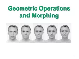
Geometric Operations and Morphing
Geometric Transformation • Operations depend on pixel’s Coordinates. • Context free. • Independent of pixel values. (x,y) (x’,y’) I(x,y) I’(x’,y’)
(x’,y’) • Example: Translation (x,y) I(x,y) I’(x’,y’)
Forward Mapping • Forward mapping: Target Source Forward Mapping
Forward vs. Inverse Mapping • Forward mapping: • Problems with forward mapping due to sampling: • Holes (some target pixels are not populated) • Overlaps (some target pixels assigned few colors) Target Source Forward mapping
Inverse mapping: • Each target pixel assigned a single color. • Color Interpolation is required. Source Target Inverse Mapping
Example: Scaling along X • Forward mapping: • Inverse mapping: Target Source (0,0) (0,0) Target Source
Interpolation • What happens when a mapping function calculates a fractional pixel address? • Interpolation: generates a new pixel by analyzing the surrounding pixels.
Interpolation • Good interpolation techniques attempt to find an optimal balance between three undesirable artifacts: edge halos, blurring and aliasing. x4 scaling N.N Bilinear Bicubic
Nearest Neighbor Interpolation • The assign value is taken from the pixel closest to the generated location: • Advantage: • Fast • Disadvantage: • Jagged results • Discontinues results
Nearest N. Interpolation Original Image
Original Image Nearest N. Interpolation
Bilinear Interpolation • The assigned value is an intermediate value between the four nearest pixels:
Linear Interpolation • Isolating v in the above equation: ve v vw xw x xe
Bilinear Interpolation • The assign value is a weighted sum of the four nearest pixels. • Each weight is proportional to the distance from each existing pixel.
N NW V NE • The bilinear interpolation is the best fit low-degree polynomial of the form: • The pixel’s boundaries are C0 continuous (continuous values across boundaries). S SE SW
Bilinear example s t s z=15 z=7 v t 0 1 z=2 z=3 0
Nearest N. Interpolation Bilinear Interpolation
Nearest N. Interpolation Bilinear Interpolation
Bicubic Interpolation • The assign value is a weighted sum of the 4x4 nearest pixels:
How can we find the right coefficients? • Denote the pixel values Vpq {p,q=0..3} • The unknown coefficients are aij {i,j=0..3} s • We have a linear system of 16 equations with 16 coefficients. • The pixel’s boundaries are C1 continuous (continuous derivatives across boundaries). t
N.N Bilinear Bicubic
Applying the Transformation T = …… % 2x2 transformation matrix [r,c] = size(img) % create array of destination x,y coordinates [X,Y]=meshgrid(1:c,1:r); % calculate source coordinates sourceCoor = inv(T) * [X(:) Y(:) ] ‘ ; % calculate nearest neighbor interpolation Xs = round(sourceCoor(1,:)); Ys = round(sourceCoor(2,:)); indx=find(Xs<1 | Xs>r); %out of range pixels Xs(indx)=1; Ys(indx)=1; indy=find(Ys<1 | Ys>c); %out of range pixels Xs(indy)=1; Ys(indy)=1; % calculate new image newImage = img((Xs-1).*r+Ys); newImage(indx)=0; newImage(indx)=0; newImage = reshape(newImage,r,c);
Types of linear 2D transformations • Rigid(Euclidean)transformation: • Translation + Rotation (distance preserving). • Similaritytransformation: • Translation + Rotation + Uniform Scale (angle preserving). • Affinetransformation: • Translation + Rotation + Scale + Shear (parallelism preserving). • Projective transformation • Cross-ratio preserving • All above transformations are groups where Rigid Similarity Affine Projective
Homogeneous Coordinates • Homogeneous Coordinates is a mapping from Rn to Rn+1: • Note: (tx,ty,t) all correspond to the same non-homogeneous point (x,y). E.g. (2,3,1)(6,9,3) (4,6,2). • Inverse mapping:
Some 2D Transformations • Translation : • Affine transformation: • Projective transformation:
Non Linear 2D Transformations • Non linear transformations do not necessarily preserve straight lines. • Methods: • Piecewise linear transformations • Non linear parametric mapping
Non linear mapping: • Example: non linear (radial) lens distortions:
Transformation Estimation • Let: x’=fx(x,y,px) ; y’=fy(x,y,py), where px and py are vector of parameters. • If the mappings are linear in px and py the parameters can be estimated using linear regression.
Example: Affine transformation • Alternative representation:
Given k points (P1,P2,..Pk) in 2D that have been transformed to (P'1,P'2,..,P'k) by affine transformation: • How many points uniquely define the affine (projective) transformation? • How can we find the affine transformation? • What if we have more points? • What can be done if points coordinates are inaccurate?
Image Warping and Morphing • Image rectification. • Key frame animation. • Image Synthesis • Facial expression • Viewing positions Image Metamorphosis.
Cross Dissolve (pixel operations) Source Image Destination Image t cross dissolve warp + dissolve
Warping + Cross Dissolve • Warp source image towards intermediate image. • Warp destination image towards intermediate image. • Cross-dissolve the two images by taking the weighted average at each pixel. source time Cross-dissolve destination warping images
warp Cross-dissolve Cross-dissolve warp
Image Metamorphosis • Let S,T be the source and the target images • Let G(p) be the transformation from S towards T, where G(0)=I the identity transformation • Let t[0,1] the time step to be synthesized Algorithm: • Warp S towards T: • Warp T toward S: • Cross dissolve:
t sourse S(t)=G(tp){S} I(t)=(1-t)S(t)+t(T(t)) target T(t)=G((1-t)p)-1{T}
Feature Based Morphing • Morph one shape into another shape • Use local features to define the geometric warping
Q Q’ P P’
Q Q’ P’ P
Q Q’ P’ P
Q Q’ P’ P
Q Q’ P’ P
Q Q’ P’ P
Q’ Q R R’ P P’ Source Image Dest Image One Segment Warping • [0,1] is the relative position along the segment (P’,Q’). • is the actual perpendicular distance to the segment. • (u’,v’) is the local coordinates of the segment (P’,Q’): • u’ is a unit vector parallel to Q’-P’ • v’ is the unit vector perpendicular to Q’-P’ v u u’ v’