Download
1 / 34
350 likes | 563 Vues
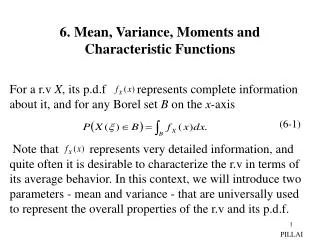
6. Mean, Variance, Moments and Characteristic Functions. For a r.v X , its p.d.f represents complete information about it, and for any Borel set B on the x -axis

E N D
6. Mean, Variance, Moments and Characteristic Functions For a r.v X, its p.d.f represents complete information about it, and for any Borel set B on the x-axis Note that represents very detailed information, and quite often it is desirable to characterize the r.v in terms of its average behavior. In this context, we will introduce two parameters - mean and variance - that are universally used to represent the overall properties of the r.v and its p.d.f. (6-1) PILLAI
Mean or the Expected Value of a r.v X is defined as If X is a discrete-type r.v, then using (3-25) we get Mean represents the average (mean) value of the r.v in a very large number of trials. For example if then using (3-31) , is the midpoint of the interval (a,b). (6-2) (6-3) (6-4) PILLAI
On the other hand if X is exponential with parameter as in (3-32), then implying that the parameter in (3-32) represents the mean value of the exponential r.v. Similarly if X is Poisson with parameter as in (3-45), using (6-3), we get Thus the parameter in (3-45) also represents the mean of the Poisson r.v. (6-5) (6-6) PILLAI
In a similar manner, if X is binomial as in (3-44), then its mean is given by Thus np represents the mean of the binomial r.v in (3-44). For the normal r.v in (3-29), (6-7) (6-8) PILLAI
Thus the first parameter in is in fact the mean of the Gaussian r.v X. Given suppose defines a new r.v with p.d.f Then from the previous discussion, the new r.v Y has a mean given by (see (6-2)) From (6-9), it appears that to determine we need to determine However this is not the case if only is the quantity of interest. Recall that for any y, where represent the multiple solutions of the equation But(6-10) can be rewritten as (6-9) (6-10) (6-11) PILLAI
where the terms form nonoverlapping intervals. Hence and hence as y covers the entire y-axis, the corresponding x’s are nonoverlapping, and they cover the entire x-axis. Hence, in the limit as integrating both sides of (6-12), we get the useful formula In the discrete case, (6-13) reduces to From (6-13)-(6-14), is not required to evaluate for We can use (6-14) to determine the mean of where X is a Poisson r.v. Using (3-45) (6-12) (6-13) (6-14) PILLAI
(6-15) In general, is known as the kth moment of r.v X. Thus if its second moment is given by (6-15). PILLAI
Mean alone will not be able to truly represent the p.d.f of any r.v. To illustrate this, consider the following scenario: Consider two Gaussian r.vs and Both of them have the same mean However, as Fig. 6.1 shows, their p.d.fs are quite different. One is more concentrated around the mean, whereas the other one has a wider spread. Clearly, we need atleast an additional parameter to measure this spread around the mean! (b) (a) Fig.6.1 PILLAI
For a r.v X with mean represents the deviation of the r.v from its mean. Since this deviation can be either positive or negative, consider the quantity and its average value represents the average mean square deviation of X around its mean. Define With and using (6-13) we get is known as the variance of the r.v X, and its square root is known as the standard deviation of X. Note that the standard deviation represents the root mean square spread of the r.v X around its mean (6-16) (6-17) PILLAI
Expanding (6-17) and using the linearity of the integrals, we get Alternatively, we can use (6-18) to compute Thus , for example, returning back to the Poisson r.v in (3-45), using (6-6) and (6-15), we get Thus for a Poisson r.v, mean and variance are both equal to its parameter (6-18) (6-19) PILLAI
To determine the variance of the normal r.v we can use (6-16). Thus from (3-29) To simplify (6-20), we can make use of the identity for a normal p.d.f. This gives Differentiating both sides of (6-21) with respect to we get or (6-20) (6-21) (6-22) PILLAI
which represents the in (6-20). Thus for a normal r.v as in (3-29) and the second parameter in infact represents the variance of the Gaussian r.v. As Fig. 6.1 shows the larger the the larger the spread of the p.d.f around its mean. Thus as the variance of a r.v tends to zero, it will begin to concentrate more and more around the mean ultimately behaving like a constant. Moments: As remarked earlier, in general are known as the moments of the r.v X, and (6-23) (6-24) PILLAI
(6-25) are known as the central moments of X. Clearly, the mean and the variance It is easy to relate and Infact In general, the quantities are known as the generalized moments of X about a, and are known as the absolute moments of X. (6-26) (6-27) (6-28) PILLAI
For example, if then it can be shown that Direct use of (6-2), (6-13) or (6-14) is often a tedious procedure to compute the mean and variance, and in this context, the notion of the characteristic function can be quite helpful. Characteristic Function The characteristic function of a r.v X is defined as (6-29) (6-30) PILLAI
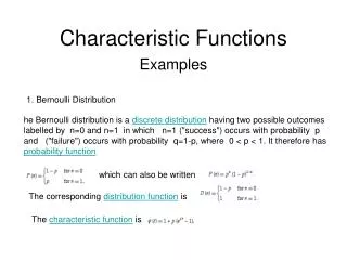
(6-31) Thus and for all For discrete r.vs the characteristic function reduces to Thus for example, if as in (3-45), then its characteristic function is given by Similarly, if X is a binomial r.v as in (3-44), its characteristic function is given by (6-32) (6-33) (6-34) PILLAI
To illustrate the usefulness of the characteristic function of a r.v in computing its moments, first it is necessary to derive the relationship between them. Towards this, from (6-31) Taking the first derivative of (6-35) with respect to , and letting it to be equal to zero, we get Similarly, the second derivative of (6-35) gives (6-35) (6-36) (6-37) PILLAI
and repeating this procedure k times, we obtain the kth moment of X to be We can use (6-36)-(6-38) to compute the mean, variance and other higher order moments of any r.v X. For example, if then from (6-33) so that from (6-36) which agrees with (6-6). Differentiating (6-39) one more time, we get (6-38) (6-39) (6-40) PILLAI
(6-41) so that from (6-37) which again agrees with (6-15). Notice that compared to the tedious calculations in (6-6) and (6-15), the efforts involved in (6-39) and (6-41) are very minimal. We can use the characteristic function of the binomial r.v B(n, p) in (6-34) to obtain its variance. Direct differentiation of (6-34) gives so that from (6-36), as in (6-7). (6-42) (6-43) PILLAI
One more differentiation of (6-43) yields and using (6-37), we obtain the second moment of the binomial r.v to be Together with (6-7), (6-18) and (6-45), we obtain the variance of the binomial r.v to be To obtain the characteristic function of the Gaussian r.v, we can make use of (6-31). Thus if then (6-44) (6-45) (6-46) PILLAI
(6-47) Notice that the characteristic function of a Gaussian r.v itself has the “Gaussian” bell shape. Thus if then and (6-48) (6-49) PILLAI
(b) (a) Fig. 6.2 From Fig. 6.2, the reverse roles of in and are noteworthy In some cases, mean and variance may not exist. For example, consider the Cauchy r.v defined in (3-39). With clearly diverges to infinity. Similarly (6-50) PILLAI
(6-51) To compute (6-51), let us examine its one sided factor With indicating that the double sided integral in (6-51) does not converge and is undefined. From (6-50)-(6-52), the mean and variance of a Cauchy r.v are undefined. We conclude this section with a bound that estimates the dispersion of the r.v beyond a certain interval centered around its mean. Since measures the dispersion of (6-52) PILLAI
the r.v X around its mean , we expect this bound to depend on as well. Chebychev Inequality Consider an interval of width 2 symmetrically centered around its mean as in Fig. 6.3. What is the probability that X falls outside this interval? We need (6-53) Fig. 6.3 PILLAI
To compute this probability, we can start with the definition of From (6-54), we obtain the desired probability to be and (6-55) is known as the chebychev inequality. Interestingly, to compute the above probability bound the knowledge of is not necessary. We only need the variance of the r.v. In particular with in (6-55) we obtain (6-54) (6-55) (6-56) PILLAI
Thus with we get the probability of X being outside the 3 interval around its mean to be 0.111 for any r.v. Obviously this cannot be a tight bound as it includes all r.vs. For example, in the case of a Gaussian r.v, from Table 4.1 which is much tighter than that given by (6-56). Chebychev inequality always underestimates the exact probability. (6-57) PILLAI
Moment Identities : Suppose X is a discrete random variable that takes only nonnegative integer values. i.e., Then similarly (6-58) PILLAI
which gives (6-59) PILLAI
Birthday Pairing • A group of n people • A) the probability that two or more persons will have the same birthday? • B) the probability that someone in the group will have the birthday that matches yours? • Solution: • C=“no two persons have the same birthday”
For n=23, • D=“a person not matching your birthday”
Equations (6-58) – (6-59) are at times quite useful in simplifying calculations. For example, referring to the Birthday Pairing Problem [Example 2-20., Text], let X represent the minimum number of people in a group for a birthday pair to occur. The probability that “the first n people selected from that group have different birthdays” is given by [P(B) in page 39, Text] But the event the “the first n people selected have PILLAI
different birthdays” is the same as the event “ X > n.” Hence Using (6-58), this gives the mean value of X to be Similarly using (6-59) we get (6-60) PILLAI
Thus PILLAI
which gives Since the standard deviation is quite high compared to the mean value, the actual number of people required for a birthday coincidence could be anywhere from 25 to 40. Identities similar to (6-58)-(6-59) can be derived in the case of continuous random variables as well. For example, if X is a nonnegative random variable with density function fX(x) and distribution function FX(X), then (6-61) PILLAI
where Similarly