Turbulence Modeling Lecture on Wall Functions and Project Discussions
Explore wall functions in boundary layer flows, integration constants, Von Karman's constant, K-e turbulence model, LES vs. RANS simulations, and modeling particle dispersion in cough simulations. Project topics cover airflow simulations, ventilation, and more.

Turbulence Modeling Lecture on Wall Functions and Project Discussions
E N D
Presentation Transcript
Lecture Objectives • Review wall functions • Discuss: Project 1, HW2, and HW3 • Project topics
Surface boundary conditions and log-wall functions E is the integration constant and y* is a length scale Friction velocity Correction y*=(n/Vt) k- von Karman's constant The assumption of ‘constant shear stress’ is used here. Constants k = 0.41 and E = 8.43 fit well to a range of boundary layer flows.
K-e turbulence model in boundary layer Wall shear stress V Eddy viscosity Wall function for e Wall function for k
HW2 • Problem 1 • Problem 2 • K- RNG vs. LES vs. DNS
DNS • Example from the previous project class Boundary conditions !
LES vs. RANS • Examples form the ongoing project
What do you see with LES Velocity Vorticity
Calculation time cost • Modeling of unsteady cough and particle dispersion • - period of 1 minute • mesh size: 500,000; particle #: 600,000; time step: 0.001s • Computers: 4 core 3.4 MHz 1) RANS Cough + particle injection (1s) Steady state calculation of background flow Particle dispersion (60 s) Conversion to unsteady 6-12 hours 3-6 hours 24-48 hours Calculation Time (2-5 day) 2) LES RANS to get Steady state background flow LES calculation to get fully developed turbulent flow (calculation of 1500 seconds) LES+part. inject (1s) LES+part. dispersion (60 s) 3-6 hours 2-3 weeks 1~2 weeks Calculation Time (2-4 weeks) 10
Comparison: Velocity LES RANS Measurements
Comparison: Cumulative Exposure 7 micron particles
HW3 • Questions?
Project 1 Airpak; How to : • Define occupancy zone • Zero diffusion • Refine mesh • Define isosurface • ….
Final project topics • You will define the project topic • Examples from previous years • Single side natural ventilation • Atrium ventilation - design problem • Rain water collection • Ventilation effectiveness – parametric study • Surface convection • Surface mass transfer