Download

1 / 41
410 likes | 600 Vues
An introduction to data assimilation Xiang-Yu Huang Danish Meteorological Institute, Denmark. Outline of the presentation. Operational NWP activities Observations and preprocessing There are still many observations we are not able to assimilate.

E N D
An introduction to data assimilation Xiang-Yu Huang Danish Meteorological Institute, Denmark
Outline of the presentation • Operational NWP activities • Observations and preprocessing • There are still many observations we are not able to assimilate. • We have to prepare for new observations to come. • Observation operators H • Error covariances B and R • They determine the assimilation quality. • We can only guess what they should be. • Data impact • It can take decades of hard work just to assimilate one data type. • How to assess data impact is application dependent. • Summary and our near future plan.
DMI-HIRLAM The operational system consists of three nested models named "G", "E" and "D".
SYNOP SHIP BUOY
AIREP AMDAR ACARS
TEMP PILOT
Comments (I):Observations alone are not enough. • Observations only cover part of the model domain (for limited area models they could also be outside of the model domain). • Some observations provide incomplete model state at given locations (e.g. only wind). • Some observations are not NWP model variables (e.g. radiance). NWP is not the only purpose of making observations.
Quality controlObserving systems have problems. • Bad reporting practice check • Blacklist check • Gross check (against some limits) • Background (short-range forecasts) check • “Buddy check” (against nearby observations) • Redundancy check • Analysis check: OI check or VarQC
Received Assimilated
Comments (II):We are far from using all the observations. • Data quality dependent. • Observing system dependent. • NWP model (resolution) dependent. • Assimilation method dependent. At the same time, we have to prepare for the new data like RO to come.
Routine monitoring Short-range forecasts - observations
Analysis methods • Empirical methods • Successive Correction Method (SCM) • Nudging • Physical Initialisation (PI), Latent Heat Nudging (LHN) • Statistical methods • Optimal Interpolation (OI) • 3-Dimensional VARiational data assimilation (3DVAR) • 4-Dimensional VARiational data assimilation (4DVAR) • Advanced methods • Extended Kalman Filter (EKF) • Ensemble Kalman Filter (EnFK)
Variational methods dx (new) (initial condition for NWP) (old forecast)
Important issues • H observation operator, including the tangent linear operator H and the adjoint operator HT. • M forecast model, including the tangent linear model M and adjoint model MT. • B background error covariance (NxN matrix). • R observation error covariance which includes the representative error (MxM matrix).
Observation operator H: from model state x to observations y This is mainly for conventional “point” observations. Horizontal and vertical integration (not interpolation) may be needed for most remote sensing data.
Examples of specific observation operators • For direct model variable observations, Hspec = I. • Radial winds: • Integrated water vapour: • Refractivity: • For radiance data, RTTOV-7 (a complicated software).
Level of preprocessing and the observation operator Hspec=HFHGHRHN Raw data: Phase and amplitude Frequency relations Ionosphere corrected observables Hspec=HGHRHN Geometry Hspec=HRHN Bending angle profiles Abel trasform or ray tracing Hspec=HN Refractivity profiles Hydrostatic equlibrium and equation of state Hspec=I Temperature profiles
Basic assumptions • Observations are unbiased. (Bias removed.) • Background is unbiased. (Bias removed?) • Observation error covariance matrix is known. R • Background error covariance matrix is known. B • Observation errors and background errors are not correlated.
Observation errors, computed for GPS/MET geopotential data (using ECMWF analyses as “TRUTH”)
Estimate B without “TRUTH” • The NMC method • Background error covariances are proportional to correlations of differences between 48 h and 24 h forecasts valid at the same time. • The analysis ensemble method • Several analyses are performed with perturbed observations. Differences between background fields are used to estimate background error covariances.
The Hollingsworth-Lönnberg method. (Estimate both B and R without “TRUTH”) B: R:
ZU ZV ZZ VU VV VZ UU UV UZ Horizontal multivariate correlation: spread the information
Wave number Vertical correlation (spread the information) for the temperature at 500 hPa Pressure (hPa)
Comments (III)We need to estimate observation errors now and then. • Observation errors include representative errors. • Observation errors should be estimated for each model system. • Observation errors may need to be re-estimated for each model refinement and instrument improvement. • (It is believed that it is more important to get o /b right than to estimate o and b.)
Comments (IV)We need to estimate the background errors again and again. • Spread information (but could also cause “problems”) • horizontally • vertically • to other variables • Impose balances to the analysis. • Background errors should be estimated for each model system and be re-estimated for each model improvement. • (It is believed that it is more important to get o /b right than to estimate o and b.)
From research to operations • Development and simple checks • Coding • Analysis increments • Case studies • Extensive experiments (e.g. one month for each season) • “Standard scores”: bias, rms, correlation, etc. • Special scores: precipitation, surface fluxes, etc. • Special aspects: noise, spin-up, etc. • Pre-operational tests • Operational use (feedback to further research)
MSLP Z850 T850 V850 T02M Z500 T500 V500 V10M Z200 T200 V200 RH850 RH500 Observation verification against EWGLAM station list Jan 2003 NOA (No ATOVS) WIA (With ATOVS) ATOVS into DMI OPR since 2002. (A) TOVS work started in 1988 (Gustafsson and Svensson)
Observed and predicted (+12h) precipitation Observed Without ZTD With ZTD
Recent HIRLAM impact studies 1. EWP: minor positive impact; blacklisting and bias correction may be needed. 2. MODIS wind: slightly negative; obs errors, screening procedures and level assignment need to be investigated. 3. MODIS IWV: neutral obsver, but positive on heavy precip cases. 4. GPS ZTD: neutral impact on most meteorological parameters, but positive impact on heavy precipitation cases. 5. AMSU-A: positive impact for the recent two-month experiment. The firstguess check is important. 6. Quikscat: positive impact
Comments (V)We need to assess data impact regularly. • It can take years and decades for an observing system to reach the operational status. • An observing system in operational use may also become redundant due to advances in assimilation techniques, new observing systems and improvements in other components. • Continuous monitoring and further tuning are necessary to keep an observing system in the operational use.
Other important aspects • Balanced motion • Adjustment and initialisation • Flow dependent B • Non-Gaussian statistics
Summary • Observations alone are not enough. • We are far from using all the available observations, and at the same time we have to prepare for the new data to come. • The “statistics” is evolving: • Observational errors • Background errors • It is getting more difficult for a new observing system to have a positive impact, as • NWP models become better • Other existing observing systems become better
Assimilating Radio Occultation data • Global data coverage. • Good vertical resolution (in contrast to most other satellite data). • Insensitive to cloud and precipitation. • Positive impact from real data collected from a single LEO has already been found on one of the most advanced data assimilation systems. We will start soon after this workshop - next week!