Download

1 / 20
220 likes | 359 Vues
This introductory lecture covers the concept of data assimilation, its application in geosciences, essential mathematical principles, and various methods used. Topics include indirect observations, errors, model parameters, and challenges in the field. Reference materials and practical examples are provided.

E N D
An introduction to data assimilation for the geosciences Ross Bannister Amos Lawless Alison Fowler National Centre for Earth Observation School of Mathematics and Physical Sciences University of Reading Introductory lecture (B) Variational intro + practical (C) Kalman filter + practical DA ‘surgery’
What is data assimilation? What is the temperature, T, of the fluid inside each jar as a function of time, t? A B
What is data assimilation? Data assimilation is concerned with how we combine these pieces of information to obtain the best possible knowledge of the system as a function of time. Gaussian with std dev. σ =√<ε2> Note on uncertainty: probability possible value (observed or modelled) “All models are wrong …” (George Box) “All models are wrong and all observations are inaccurate” (a data assimilator)
What is data assimilation? xf(t1) xa(t2) xa(t1) = observation start of the system xtrue(t) (unknown) xf(t3) time This is an example of a ‘filter’ • Data assimilation has: • prediction stages (xf = ‘forecast’, ‘prior’, ‘background’) • analysis stages (xa) (extrapolation) (interpolation) xf(t2)
What is data assimilation? “[The atmosphere] is a chaotic system in which errors introduced into the system can grow with time … As a consequence, data assimilation is a struggle between chaotic destruction of knowledge and its restoration by new observations.” Leith (1993)
Outline and references What is data assimilation? Applications of data assimilation in the geosciences A prototype data assimilation system Indirect observations and prior knowledge Errors Leading data assimilation methods Essential mathematics Challenges, subtleties, caveats, … • References: • Kalnay, 2003, Atmospheric Modeling, Data Assimilation and Predictability. • Daley, 1991, Atmospheric Data Analysis. • Lorenc, 2003, The potential of the ensemble Kalman Filter for NWP – a comparison with 4d-Var, QJRMS 129, 3183-3203. • van Leeuwen, Particle filtering in geophysical systems. • Rodgers , 2000, Inverse methods for atmospheric sounding, theory and practice, World Scientific, Singapore. • Wang X., Snyder C., Hamill T.M., 2007, On the theoretical equivalence of differently proposed ensemble-3D-Var hybrid analysis schemes, Mon. Wea. Rev. 135. pp. 222-227.
Applications of data assimilation in the geosciences Atmospheric retrievals Atmospheric dynamics / NWP Reanalysis L L Parameter estimation Inverse modelling for sources/sinks α, β, γ Hydrological cycle H Oceanography Carbon cycle Atmospheric chemistry
A prototype data assimilation problem Combining imperfect data Consider two sources of information (e.g. measurements), x1 ± σ1and x2 ± σ2that each estimate x (assume Gaussian statistics) pn(xn|x) δxn : “the probability that the data xn lies between xn and xn+δxn given that the ‘true’ value is x” The joint probability is p1(x1|x) δx1 p2(x2|x) δx2(“the probability that x1 is … and x2 is … given x”) In the above theory, x is known and x1 and x2 are unknown. Now introduce actual information x1 and x2 : now x1 and x2 are known and x is unknown. What x maximizes p(x1, x2|x)?
A prototype data assimilation problem Combining imperfect data What xmaximizesp(x1, x2|x)? The same x that minimizes the ‘cost function’ To minimize, look for stationary values of I: If information source 2 is much more accurate than information source 1, then σ2 << σ1: If information source 1 is much more accurate than information source 2, then σ1 << σ2:
Indirect observations and prior information If x1 and x2 were measurements, they are direct measurements of x. Many observations are indirect. E.g. • Generalise: • x is the state vector (n elements) • ymo is the model’s version of the observations (mo=“model observations”) (p elements) • h is the forward model or observation operator (input n elements, output p elements) • y is the observation vector (p elements) • Strategy: what x gives best fit between y and ymo?
Indirect observations and prior information model parameters The structure of the state vector (for the example of meteorological fields u, v, θ, p, q are 3-D fields; λ, φ and ℓ are longitude, latitude and vertical level). There are n elements in total. The observation vector – comprising each observation made. There are p observations.
Indirect observations and prior information • Examples of h • For in-situ observations, h is an interpolation function. • For radiance observations, h is a radiative transfer operator. • For observations at a later time than that of x, h includes a forecast model. • Prior information • Often the observations are insufficient to determine x. • Introduce prior information (a-priori, background, first guess, forecast), xf. • One strategy (variational assimilation) to solving the assimilation problem is to ask: • “What x (called xa [in earlier slide this was called xe]) gives: • ymo that is the closest possible to y and • x that is the closest possible to xf?” • Construct a cost functional and minimize w.r.t. x • (a generalized least-squares problem).
Indirect observations and prior information Square of length of vector • Error covariance matrices define the norm (these respect the uncertainty of xf and y and are important!) • Pf forecast (or background) error covariance matrix (n × n matrix). Sometimes called B. • R observation error covariance matrix (p × p matrix). • This cost function • can be derived from Bayes’ Theorem by assuming forecast and obs errors obey Gaussian stats, • has argument, x (think of as a control variable), • may be extended to include fit to other unknowns in the system (e.g. the fact that h is imperfect, including model parameters.
Errrors everywhere All significant sources of uncertainty should be accounted for in data assimilation Example 1 – repeated observations of air temperature • Random errors: • background (a-priori) errors • observation errors • model errors • representivity errors • Systematic errors: • biases in background • biases in observations • biases in model y (T observations) unbiased thermometer truth truth biased thermometer Example 2 – representivity errors due to model grid
Leading methods of solving the DA problem Variational-type approach Kalman filter-type approach (linear obs operator, Htxt= ht(xt) ← analysis update at time t ← analysis error covariance ← forecast ← forecast error covariance Linear forecast model Model error covariance matrix
Leading methods of solving the da problem Ensemble Kalman filter-type approach Have N ensemble members (index i, 1 ≤ i ≤ N). Differences between them represent uncertainty. Approximate the forecast error covariance matrix with an ensemble to make manageable the Kalman update equation for n << p A superposition of ensemble members But beware ...
Mathematics required • Vector representation of fields • Matrix algebra • Linear vector spaces • Matrix inversion • Vector derivative • Generalized chain rule • Jacobians • Eigenvectors/eigenvalues • Singular vectors/values • Variances, covariances, correlations • Matrix rank • Lagrange multipliers www.met.reading.ac.uk/~ross/MTMD02/MathTools.pdf
Summary of basic principles • DA is concerned with estimating the state of a system given: • observations (direct [e.g. in-situ] and indirect [e.g. remotely sensed]), • forecast models (to provide a-priori data, given too-few obs), • observation operators (to connect model state with obs). • All data have uncertainties, which must be quantified. • DA estimates are sensitive to uncertainty characteristics, which are often poorly known. • Many observations and model have systematic as well as random errors. • Should take into account all sources of error in the system. • DA theory is suited mostly to errors that are Gaussian distributed. • Most errors are non-Gaussian and non-linearity is synonymous with non-Gaussianity. • DA problems are computationally expensive and require intensive development effort.
Some subtleties and caveats of DA • DA estimates are not the ‘truth’ and can be problematic for some kinds of analyses: • A good fit to observations does not guarantee that the analysis is correct! • E.g. if h-operator has inadequacies not accounted for, or if error covariances matrices are poor. • Unobserved parts of the system may be poor. • E.g. in meteorology, horizontal winds may be constrained well by obs, but implied vertical wind may be poor. • Assimilated fields may be subject to other constraints: • E.g. certain balance constraints. • Be careful with error covariance matrices: • Pf, R need to be tuned for variational DA, Pf subject to sampling problems for ensemble DA. • DA systems should be well tested before using real data: • Test h-operators (forecast models and obs. operators) – which parts of x is ymo sensitive to? • Adjoint tests, H, HT if using variational data assimilation. • Test DA system with simulated obs. from a made-up truth (identical twin experiments). • For assimilation of real data, validate analysis against independent obs. if possible.