
Hydrologic Ensemble Post-Processor: An Overview
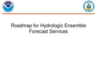
Hydrologic Ensemble Post-Processor: An Overview. Elements of a Hydrologic Ensemble Prediction System. Ensemble Verification System. QPE, QTE, Soil Moisture. QPF, QTF. Ensemble Pre-Processor. Parametric Uncertainty Processor. Data Assimilator. Hydrology & Water Resources Models.

Hydrologic Ensemble Post-Processor: An Overview
E N D
Presentation Transcript
Elements of a Hydrologic Ensemble Prediction System Ensemble Verification System QPE, QTE, Soil Moisture QPF, QTF Ensemble Pre-Processor Parametric Uncertainty Processor Data Assimilator Hydrology & Water Resources Models Streamflow Ensemble Hydrograph Post-Processor Hydrology & Water Resources Ensemble Product Generator Ensemble Product Post-Processor Fig 1
Need for Hydrologic Ensemble Post-Processing • ESP forecasts are conditioned on an ensemble of precipitation and temperature forecasts (i.e. ysim|fcst). • If the input P &T ensemble members are “properly calibrated” they will have the same long-term climatology as the historical P & T used for hydrologic model calibration. • Climatological ESP runs using the historical data, by construction, use P & T that are “properly calibrated”. • This means that problems with the hydrologic ensemble forecasts are due to “hydrologic model bias and uncertainty” if input forcing is “properly calibrated”. • Hydrologic model bias and uncertainty occur because: • Hydrologic model simulations cannot produce hydrologic products that are always completely unbiased. • Current ESP forecasts assume that the initial conditions are known. This causes the ESP spread to be underestimated, especially for forecast periods with little P & T forcing variability. • Hydrologic model simulations do not account for hydrologic model error (structure and parameters). This also causes the ESP spread to be underestimated.
Russian River • Total Area 3465 km2. • Elevation 17m - 1245m. • 2 Flood Control Reservoirs • Upstream Diversions • 3 Local Areas. • 3 Official Flood Forecast Points. • Floods Nearly Every Year. • 3 Major Floods in Past 40 Years. Hydrologic hydrograph post-processing is needed at the output of each forecast segment where streamflow measurements have ever been made. Adjusted hydrographs need to be routed and used as input downstream. Calibration of post-processors needs to proceed from upstream to downstream. Hydrologic hindcasting needs to include hydrologic post-processing.
Post-Processing goal is to answer the question: • If input time series P,T were to occur, what time series, Qobs, would be measured? • Post-Processing Approach is: • Use hydrologic model to compute Qsim(P,T). • Map Qsim(P,T) into an ensemble of equally-likely estimates of Qobs(P,T) that account for “predictive uncertainty”.
Hydrologic Ensemble Post-Processor(to correct raw ESP bias and spread errors) General Linear Model Hydrologic Post-Processor (GLM-PostP) Raw ESP Streamflow Ensemble Hydrographs Adjusted ESP Streamflow Ensemble Hydrographs • This post-processor operates on hydrologic model output hydrograph(s) for a prescribed period of time. This may be a single hydrograph that is a model simulation based on observed MAP/MAT values or a set of raw ESP ensemble hydrograph members. • This post-processor attempts to produce adjusted hydrographs that: • Preserve the “skill” of the raw model hydrograph • Removes mean bias • Produces an ensemble of members that represent in an “equally-likely” sense the observed hydrograph that is being predicted • Preserves temporal scale dependency relationships
Product Post-Processor Qsim and Qobs are scalar variables Use NQT to transform to qsim and qobs Assume qsim and qobs are bivariate normal RV’s Generate sample values of qobs|qsim (scalar values) and use inverse NQT to get corresponding values of Qobs|Qsim Hydrograph Post-Processor Qsim and Qobs are vector variables Use NQT to transform elements of Qsim and Qobs to qsim and qobs Assume qsim and qobs are multivariate normal RV’s Generate sample values of qobs|qsim (vector values) and use inverse NQT to get corresponding values of Qobs|Qsim Product vs HydrographPost-Processing
qobs qsim Qobs Qsim Normal Quantile Transformation Data Transformations Data transformation may be very helpful to keep hydrologic post-processors both simple and “effective”. The work reported in this presentation uses an empirical CDF for observed and simulated flow and a NQT to transform the observed or simulated flow to a standard normal deviate. Note: Parameters of NQT vary with day-of-year. Different parameters are used for each day. Also, the NQT uses the empirical climatological distributions of Qobs and Qsim
Hydrograph Post-ProcessorData Window Analysis Period Future Period Qobsa (given) Qsima (given) Qobsf (to be predicted) Qsimf (given) Time Na Nf Nw = Na + Nf “Present” (t = 0) Variables Qobsa, Qobsf, Qsima and Qsimf are vectors whose elements form time-series of observed and simulated hydrograph components in the analysis (a) and future periods (b). (Note: The value of Na can be = 0).
Vector Hydrograph Post-Processor The objective is to generate an ensemble of values of the vector Z1 = [Qobsf], given the vector values of Z2 = [Qsimf, Qobsa and Qsima]. We wish to create Z1.2 = Z1 | Z2. To do this, we use the General Linear Model: Vector Definitions:
General Linear Model:Covariance Matricies Covariance Matrix of Vector Z (zero mean): Partition Z into Z1 and Z2: Partitioned Covariance Matrix:
General Linear Model Parameter Estimation Note: The elements of Z have marginal distributions with zero mean. The relationships for A and B apply to any random variable and give least-square estimates of the elements of Z1.2.
Control GLM-PostP Calibration Qesp(1…Nf) Qsim(-Na…0) Qobs(-Na…0) Qsim Qobs GLM-PostP GLM-PostP Ensemble of Adjusted Simulated Hydrographs f(Qobs|Qsim) Adjusted ESP Hydrographs f(Qobs|fcst) Qsim(-Na…Nf) Qobs(-Na…Nf) GLM Hydrologic PostProcessor GLM-PostP “Parameters” Simulation Option ESP Option
Calibration Process • Define Data Processing Window • Assemble historical Qobs and Qsim daily data into separate arrays, each of size Nobs x Nw where • Nw = Na + nf • Nobs = Nyrs * Nbuffer • For each day in the data window (-Na … Nf) • Estimate daily empirical CDF’s of Qobs and Qsim • Use empirical CDF to map • Qobs => qobs ~ N(0,1) • Qsim => qsim ~ N(0,1) • Assume qobs and qsim are pairwise bivariate normally distributed for all possible pairs • Form Z = [Z1 Z2]T • Estimate covariance matrix of Z • Estimate A and B
Historical Data Processing Select historical data from each year from a window of N days where N = Na + Nf + Nbuffer Analysis Period Future Period Qobsf (to be predicted) Qsimf (given) Qobsa (given) Qsima (given) Time Na Nf Buffer Buffer Nw = Na + Nf “Present” (t = 0) Note: Nbuffer sets of Nw days of data are taken from each of NYRS years of data. This gives NOBS = NYRS * Nbuffer observations for each day
GLM Calibration Control Data • Specify Segment ID (e.g. CREC1) • Specify Calibration Period • Starting year • Ending year • Define Data Window • Specify Day-of-year (mm/dd) • Specify Model Window: • Nf = Duration of future period • Na = Duration of analysis period • Specify Buffer Size (Nbuffer)


![[Post Processor]](https://cdn2.slideserve.com/5127715/slide1-dt.jpg)