Download
1 / 11
110 likes | 342 Vues
Semi- Lagrangian Dynamics in GFS. Sajal K. Kar. Introduction. Over the years, the accuracy of medium-range forecasts has steadily improved with increasing resolution at the ECMWF. Introduction of the semi- Lagrangian (SL) treatment of advection has been recognized as a contributing factor.

E N D
Semi-Lagrangian Dynamics in GFS Sajal K. Kar
Introduction • Over the years, the accuracy of medium-range forecasts has steadily improved with increasing resolution at the ECMWF. Introduction of the semi-Lagrangian (SL) treatment of advection has been recognized as a contributing factor. • An SL scheme for advection, compared to an Eulerian scheme, allows larger time steps, thus improving model efficiency, particularly at high resolutions. • Joe Sela and colleagues developed a semi-Lagrangian semi-implicit (SLSI) version of the Eulerian-SI (operational) GFS. The numerical schemes used broadly follow the ECMWF approach. NEMS/GFS Modeling Summer School
Some details of SL GFS • Hydrostatic shallow-atmosphere primitive equations in terrain-following s-p hybrid vertical coordinate on Lorenz grid. • Prognostic field variables include u, v, Tv, lnps, q, and a few other tracers. • Vertical finite-difference scheme designed to conserve angular momentum and total energy. • Governing equations are space-time discretized using the SLSI-SETTLS scheme. SETTLS stands for the Stable-Extrapolation Two-Time-Level Scheme (Hortal 2002, QJRMS), which will be reviewed later. NEMS/GFS Modeling Summer School
More details of SL GFS • The ECMWF model employs a quasi-cubic Lagrange-polynomial 3D interpolation for the prognostic fields, whereas a tri-linear interpolation is used for the other rhs terms. • The SL GFS includes options of (i) Hermite-, (ii) quasi-cubic Lagrange-polynomial 3D interpolations used for all fields to be interpolated. • ECMWF model employs finite-elements and SL employs finite-difference in the vertical. • Recently, we have added options of a SETTLS based departure-point scheme and a ‘modified Lagrange’ interpolation scheme that mimics the ECMWF. NEMS/GFS Modeling Summer School
Semi-Lagrangian vs. Eulerian • The SLSI-SETTLS scheme, compared to the Eulerian time-filtered-leapfrog-SI scheme, is a two time-level scheme. Thus, the SL model does not need a time filter and is relatively more efficient. • Overhead of the SL scheme comes from the departure-point calculations and 3D/2D interpolations of prognostic variables to the departure points at each time step. However, reasonably large time steps allowed by the SL scheme offsets this computational overhead. • For example, T574 Eulerian GFS, equivalent grid-resolution 27 km, uses a time step of 180 s. The SL GFS for T1534, with equivalent grid-resolution of 13 km, can use a time step of 450 s. NEMS/GFS Modeling Summer School
Semi-Lagrangian Explicit SETTLS NEMS/GFS Modeling Summer School
Details of the SETTLS Backward Trajectory: . A t + Dt M t + Dt/2 D t SETTLS uses the points, (D, t+Dt) and (A, t), to evaluate the R term at M. Also used to locate departure points. NEMS/GFS Modeling Summer School
Semi-Lagrangian Semi-Implicit SETTLS . NEMS/GFS Modeling Summer School
Updates on SL GFS • Recently, a systematic inter-comparison of 4 selected SL options in the SL-T1148 with the Eu-T574 was carried out in test runs without cycling. See details of the SL options in http://www.emc.ncep.noaa.gov/mmb/skar/Kar_GCWMB_20121129.pdf and the model inter-comparison scores in http://www.emc.ncep.noaa.gov/mmb/skar/SLG1134_options2_.pptx • Encouraged by the T1148 results and other considerations, the SL GFS (T1534-L64) is slated for operational implementation in 2014. • Preliminary test runs without cycling of SL-T1534 are being carried out. • The SL GFS is about to become a part of NEMS. NEMS/GFS Modeling Summer School
500 hPa Hgt AC for SL-T1534 (Courtesy of DaNa Carlis) NEMS/GFS Modeling Summer School
References • IFS Documentation – Cy38r1, 2012: Part III: Dynamics and numerical procedures, 1-29. • Sela, J., 2009a: The implementation of the sigma pressure hybrid coordinate into the GFS. NOAA/NCEP Office Note 461. 25 pp. • Sela, J., 2010: The derivation of the sigma pressure hybrid coordinate semi-Lagrangian model equations for the GFS. NOAA/NCEP Office Note 462. 31 pp. NEMS/GFS Modeling Summer School