Download
1 / 28
280 likes | 513 Vues
One-Way ANOVA. Independent Samples. Basic Design. Grouping variable with 2 or more levels Continuous dependent/criterion variable H : 1 = 2 = ... = k Assumptions Homogeneity of variance Normality in each population. The Model. Y ij = + j + e ij , or,

E N D
One-Way ANOVA Independent Samples
Basic Design • Grouping variable with 2 or more levels • Continuous dependent/criterion variable • H: 1 = 2 = ... = k • Assumptions • Homogeneity of variance • Normality in each population
The Model • Yij = + j + eij, or, • Yij - = j + eij. • The difference between the grand mean () and the DV score of subject number i in group number j • is equal to the effect of being in treatment group number j, j, • plus error, eij
Four Methods of Teaching ANOVA Do these four samples differ enough from each other to reject the null hypothesis that type of instruction has no effect on mean test performance?
Error Variance • Use the sample data to estimate the amount of error variance in the scores. • This assumes that you have equal sample sizes. • For our data, MSE = (.5 + .5 + .5 + .5) / 4 = 0.5
Among Groups Variance • Assumes equal sample sizes • VAR(2,3,7,8) = 26 / 3 • MSA = 5 26 / 3 = 43.33 • If H is true, this also estimates error variance. • If H is false, this estimates error plus treatment variance.
F • F = MSA / MSE • If H is true, expect F = error/error = 1. • If H is false, expect
p • F = 43.33 / .5 = 86.66. • total dfin the k samples is N - 1 = 19 • treatment df is k – 1 = 3 • error df is k(n - 1) = N - k = 16 • Using the F tables in our text book,p < .01. • One-tailed test of nondirectional hypothesis
Deviation Method • SSTOT = (Yij - GM)2= (1 - 5)2 + (2 - 5)2 +...+ (9 - 5)2 = 138. • SSA = [nj (Mj - GM)2] • SSA = n (Mj - GM)2 with equal n’s= 5[(2 - 5)2 + (3 - 5)2 + (7 - 5)2 + (8 - 5)2] = 130. • SSE = (Yij - Mj)2= (1 - 2)2 + (2 - 2)2 + .... + (9 - 8)2 = 8.
Computational Method = (1 + 4 + 4 +.....+ 81) - [(1 + 2 + 2 +.....+ 9)2] N = 638 - (100)2 20 = 138. = [102 + 152 + 352 + 402] 5 - (100)2 20 = 130. SSE = SSTOT – SSA = 138 - 130 = 8.
Magnitude of Effect • Omega Square is less biased
Magnitude of Effect • Put a confidence interval on eta-squared. • http://core.ecu.edu/psyc/wuenschk/SPSS/SPSS-Programs.htm
Magnitude of Effect • Enter F and df into NoncF.sav
Magnitude of Effect • Run syntax file NoncF3.sps. • CI runs from .837 to .960.
Pairwise Comparisons and Familywise Error • fw is the alpha familywise, the conditional probability of making one or more Type I errors in a family of c comparisons. • pc is the alpha per comparison, the criterion used on each individual comparison. • Bonferroni: fwcpc
c = 6, pc = .01 • alpha familywise might be as high as 6(.01) = .06. • What can we do to lower familywise error?
Fisher’s Procedure • Also called the “Protected Test” or “Fisher’s LSD.” • Do ANOVA first. • If ANOVA not significant, stop. • If ANOVA is significant, make pairwise comparisons with t. • For k = 3, this will hold familywise error at the nominal level, but not with k > 3.
Computing t • Assuming homogeneity of variance, use the pooled error term from the ANOVA: • For A versus D:
For A versus C and B versus D: • For B versus C • For A vs B, and C vs D,
Underlining Means Display • arrange the means in ascending order • any two means underlined by the same line are not significantly different from one another Group A B C D Mean 2 37 8
The Bonferroni Procedure • Does NOT require that ANOVA be conducted or, if conducted, that ANOVA be significant. • Compute an adjusted criterion of significance to keep familywise error at desired level
For our data, • Compare each p with the adjusted criterion. • For these data, we get same results as with Fisher’s procedure. • In general, this procedure is very conservative (robs us of power).
Ryan-Einot-Gabriel-Welsch Test • Does not require a significant ANOVA. • Holds familywise error at the stated level. • Has more power than other techniques which also adequately control familywise error. • SPSS will do it for you.
Which Test Should I Use? • If k = 3, use Fisher’s Procedure • If k > 3, use REGWQ • Remember, ANOVA does not have to be significant to use REGWQ.
Teaching method significantly affected test scores, F(3, 16) = 86.66, MSE = 0.50,p < .001, 2 = .942, CI.95 = .837, .960. Pairwise comparisons were made with Bonferroni tests, holding familywise error rate at a maximum of .01. As shown in Table 1, the computer-based and devoted methods produced significantly better student performance than did the ancient and backwards methods.
Computing ANOVA From Group Means and Variances with Unequal Sample Sizes GM= pjMj =.2556(4.85) + .2331(4.61) + .2707(4.61) + .2406(4.38) = 4.616. Among Groups SS =34(4.85 ‑ 4.616)2 + 31(4.61 ‑ 4.616)2 + 36(4.61 ‑ 4.616)2 + 32(4.38 ‑ 4.616)2 = 3.646. With 3 df,MSA = 1.215, and F(3, 129) = 2.814, p = .042.