Download
1 / 31
350 likes | 544 Vues
These notes are developed from “Approaching Multivariate Analysis: A Practical Introduction” by Pat Dugard, John Todman and Harry Staines. One-way ANOVA. A study designed to investigate dosages for a new ACE-inhibitor in the treatment of hypertension.

E N D
These notes are developed from “Approaching Multivariate Analysis: A Practical Introduction” by Pat Dugard, John Todman and Harry Staines. One-way ANOVA
A study designed to investigate dosages for a new ACE-inhibitor in the treatment of hypertension. The new drug is believed to have fewer side effects than the currently favoured ACE-inhibitor. Fifty patients with systolic blood pressure (SBP) in the range 150 – 170 mm Hg are randomly allocated to one of five conditions. The independent variable is drug DOSAGE, with levels being 4mg, 6mg, 8mg, and 10mg for the new drug and 10mg for the old drug, which is known to be an effective level for that drug. The dependent variable is the drop in systolic blood pressure (SBP) one week after administration. An Example For A One-Way Design
The specific hypothesis was that SBPDROP (the dependent variable), would show an upward trend with dosage of the new drug, equalling the drop achieved by 10mg dose of the currently favoured drug somewhere in the range 4mg to 10mg used in the study. Fifty participants are randomly assigned, ten to each condition, and the data are shown in the table. An Example For A One-Way Design
Because this is a between-subjects design, the data need to be entered in just two columns, one for the independent variable (DOSAGE) and one for the dependent variable (SBPDROP), so that each participant occupies a single row. Thus, in the SBPDROP column, the data for 4mg of the new drug would be entered first and the data for 6, 8 and 10mg would be entered in turn below that, followed by the data for 10 mg of the old drug. The DOSAGE column would contain ten 1s, followed by ten 2s, ten 3s, ten 4s and ten 5s. The first and last few rows showing the data organized for entry into SPSS can be seen in the table. An Example For A One-Way Design
An Example For A One-Way Design The output will be easier to read if the five dosage/drug conditions are given their names rather than the codes 1 to 5. We can easily arrange this once the data are in the datasheet. At the bottom of the datasheet, click the Variable View tab. Now we see each of the variables listed with their properties. Each of these properties can be altered: for instance we may want to specify that 0 decimal places.
An Example For A One-Way Design Click in the Values cell for DOSAGE and a button appears: clicking this opens an SPSS Dialog Box, and here we can assign labels to each of the five levels of DOSAGE. Type 1 in the Value Box, type new4mg in the Value Label Box and click Add. Repeat with 2 and new6mg, and so on to 5 and old10mg. The dialog box is shown just before we click Add for the last time. Then click OK.
An Example For A One-Way Design To see the labels displayed in the datasheet, return to Data View using the tab at the bottom, then click View on the menu bar, then Value Labels, which toggles between displaying code numbers and labels. It may also be helpful to give the dependent variable an extended label to be used in the output. To do this, select Variable View at the bottom tab, click Label in the SPBDROP row, and write 'fall in systolic blood pressure' in the highlighted cell.
Once the data are entered, select Analyze from the menu bar, then Compare Means, then One-Way ANOVA, to get SPSS Dialog Box. Requesting The Analysis
Select SBPDROP from the variable list and use the arrow to put it in the Dependent List Box. Then put DOSAGE in the Factor Box in the same way, so the dialog Box appears as shown. Requesting The Analysis
Click the Options button to get a list of statistics for optional printing. Click the Descriptives Box to get means etc., then Homogeneity of variance test for Levene's test of equality of group variances and Means Plot. We will ignore the Contrasts and Post Hoc buttons for the moment. When we have looked at the output for the main analysis, we will return to these buttons to carry out follow-up tests. Click Continue and OK to get the main analysis. Requesting The Analysis
The test of homogeneity of variance. We may note, however, that some authors have questioned the legitimacy of Levene's test. In any case, ANOVA is quite robust to moderate departures from homogeneity unless treatment groups are small and unequal in size. In our example we see that the Levene statistic is not quite significant (the probability is 0.054, look at the Sig column), though if we had smaller and/or unequal group sizes, we might consider using the Brown-Forsythe or Welch test instead of the F test (these are available in the Options dialog box). Understanding The Output
Understanding The Output Then we get the ANOVA summary table, with the F statistic quoted and its df, and we see that the difference among the five conditions is highly significant (F(4,45) = 9.085, p < 0.001). From the summary table we can easily compute effect size as η2 = 351.52/786.82 = 0.447. This is a very large effect size, with α = 0.05, two-tailed and n = 10 per cell, the power analysis indicates that retrospective power = 1.
Understanding The Output The plot provides a graphic illustration of the means.
Understanding The Output It is obvious from the plot that there is not a steady increase with dosage of the new drug, and the drop in SBP with 10mg of the currently used drug is between those for 8mg and 10mg of the new drug. There are now several strategies available to us. We could carry out post hoc tests on the differences between all pairs of conditions, in which case we would need to deal with the problem of multiple testing. It would not be okay to just do a series of t-tests. Briefly, if we were to carry out 20 tests with alpha (the probability of a Type I error) set at 0.05 and the null hypothesis was true in every case, just by chance we might expect to find one difference significant at p < 0.05 (i.e., 1 in 20 Type I errors).
Requesting The Analysis There is a variety of procedures designed to set α for the family of tests at 0.05, and these differ in how conservative they are. One of the most commonly used is Tukey's Honestly Significant Difference (HSD) test. We will use that. We now re-do our analysis and ask for the Tukey HSD test at the same time. As before, select from the menu bar Analyze, then Compare Means, then One-Way ANOVA, but this time click the Post Hoc button to get a choice of post hoc tests. Select Tukey, then click Continue and OK to get the results of the Tukey test.
You can see that each level of DOSAGE, starting with new4mg, is compared with every other level. Understanding The Output
New4mg is first compared with new6mg, the mean difference between these levels was 0.100 with a confidence interval from -3.85 to 4.05. Since this confidence interval overlaps zero, the null hypothesis that the mean difference is zero would not be rejected. The probability (look in the Sig column) is 1.000, so it is virtually certain that the observed difference between these two levels is just random variation. Understanding The Output
This output tells us that new4mg and new6mg did not differ significantly and likewise, new8mg, new10mg and old10mg did not differ significantly from one another. On the other hand, each of new4mg and new6mg differed significantly (p < 0.05) from each of new8mg, new10mg and old10mg. Understanding The Output
Another strategy would be to carry out planned comparisons (i.e., based on hypotheses that motivated the research). One such hypothesis might be that there would be a linear trend across the five conditions. This can be tested by re-doing the one-way ANOVA, but this time click the Contrasts button to get SPSS Dialog Box. Click the Polynomial Box, and use the drop-down arrow to put Linear in the Degree Box. We are selecting the first (linear) polynomial contrast or comparison. If we wanted to test for a quadratic trend (a single curve) we would tick Polynomial and select Quadratic in the Degree Box. Requesting The Analysis
It is only possible to test up to a polynomial one less than the number of conditions (i.e., 5-1=4, in this case). In fact, if you select the 4th polynomial, you will get tests of all of the lower polynomials as well. We will do that because, as well as testing the linear trend, we can make a point about the cubic trend. Click Continue and OK to see the results of the trend tests. Requesting The Analysis
Understanding The Output In the first row, the results of the test of differences among the five conditions is repeated, then the results of the four trend tests are given. The one we were initially interested in is the planned contrast; the a priori hypothesis of a linear trend. We see that, even though the plot did not appear to be very close to a straight line, the linear trend is highly significant (F(1,45) = 28.144, p <0.001). In the following row, we learn that the deviation from the linear trend; that is, the non-linear component of the trend remaining, approaches significance (p = 0.055).
Understanding The Output There are three df for the nonlinear part of the trend, so the near significance of the p value suggests that a particular non-linear component of trend taking one of these dfs may also be significant, which tells us that a particular non-linear component of trend may also exist. In fact, the cubic trend is significant (p = 0.013), which is not surprising given that the plot shows a double (S-shaped) curve.
Understanding The Output Even though the cubic trend is significant, we would not see any point in reporting it unless we could think of some plausible (post hoc) explanation for it. In this case, a possible explanation does exist. Neither 4mg nor 6mg of the new drug is sufficient to be effective in bringing down SPB, and it could be for that reason that SBPDROP does not differ between them. Once the drug is given at the higher level of 8mg, we do see a drop in SBP, and this effect is increased at 10mg. In fact at 10mg, the new drug exceeds the effect of 10mg of the currently favoured drug, so we see S shape that we observed on the graph.
Understanding The Output Now, we need to be clear that, if we report the cubic effect, we would not be confirming a hypothesis – we would be generating a hypothesis from inspection of our data. This hypothesis would need to be tested in a new experiment. In fact for this study the most useful next step would be an investigation into just where between 8mg and 10mg of the new drug is the most useful dose. Also we would need to check on our belief that there are fewer side effects and that we have not missed an unexpected one.
There is a further situation concerning follow-up tests that we will raise. This is when we look at our data and generate a complex post hoc hypothesis that requires more than testing differences between all pairs of means (Tukey) or testing each experimental mean against a control mean (Dunnett). For example, we might generate the hypothesis that there is a threshold effect in the drug dosage, and that below this level there is no effect on SBP. Specifically, we would be hypothesizing that at least 8mg is needed to see any effect on SBP whichever ACE inhibitor we use. Requesting The Analysis
We can use the Scheffé procedure to test complex post hoc hypotheses. For the example just suggested, we would compare the mean of the first two conditions with the mean of the last three. To do this we define a contrast, which multiplies each level mean by a suitably chosen coefficient, which is just a number. For our example we compare the mean of the first two levels (new4mg and new6mg) with the mean of the last three (new8mg, new10mg and old10mg). To find the difference we need to subtract one mean from the other. The steps for assigning coefficients to the levels are listed below. Requesting The Analysis
1. Mean of first two levels = (new4mg + new6mg)/2 = ½ new4mg + ½ new6mg 2. Mean of last three levels= (new8mg + new10mg + old10mg)/3 = 1/3 new8mg + 1/3 new10mg + 1/3 old10mg 3. Contrast = 1/3 new8mg + 1/3 new10mg + 1/3 old10mg – ½ new4mg – ½ new6mg 4. Coefficients for contrast (in the same order as the levels) –½, -½, +1/3, +1/3, +1/3 The coefficients must sum to zero, and those for the means in the first set that are assumed not to differ are identical, and those for the means in the other set are also identical. You can easily see that this holds in the above case. SPSS doesn't allow us to enter fractions, and 1/3 does not have an exact decimal version. So there is a final step. 5. Multiply by the lowest common denominator (the smallest number that can be divided without a remainder by the two denominators 2 and 3, that is 6) to get all whole numbers -3, -3, 2, 2, 2. Requesting The Analysis
Requesting The Analysis The contrast we end up with is six times the one we wanted, but we shall be testing whether it is zero, so six times the original is just as good. To do this in SPSS return to SPSS Dialog Box and click the Contrasts button to get SPSS Dialog Box. Enter the first coefficient (-3) in the Coefficients Box and click Add. This is repeated for successive coefficients. The dialog box is shown just before Add is clicked for the last time. Click Continue and OK to obtain the output.
Understanding The Output We select the first or second row, depending on whether or not the Levene test indicated that we could assume equal variances. The Levene statistic was not significant so we look at the first row. We find a t15 value that is highly significant, but we do not accept the significance level given because we need to allow for the fact that we decided on the comparison after looking at our data, which is equivalent to testing all possible contrasts before looking at the data (a rather extreme form of multiple testing).
Understanding The Output Instead, we use the Scheffé correction. As the Scheffé correction works with F rather than t, we square the t-value (5.7732 = 33.33) to get F = 33.33 with 4 and 45 degrees of freedom. Now comes the adjustment. If we look up the critical value of F(4,45) in a statistical table for α set at 0.001, we get Fcrit = 5.56. The adjustment involves multiplying this critical value by the number of levels of the factor minus one (i.e., 4). So the adjusted critical value of F is 4 × 5.56 = 22.24, which is still less than our obtained value of F = 33.33, so the two sets of means differ significantly (adjusted F(4,45) = 33.33, p < 0.001) using a Scheffé correction for post hoc multiple testing.
GET FILE='12d.sav'. ← include your own directory structure c:\… DISPLAY DICTIONARY /VARIABLES dosage sbpdrop. ONEWAY sbpdrop BY dosage /STATISTICS DESCRIPTIVS HOMOGENEITY /PLOT MEANS /MISSING ANALYSIS. ONEWAY sbpdrop BY dosage /STATISTICS DESCRIPTIVS HOMOGENEITY /PLOT MEANS /MISSING ANALYSIS /POSTHOC=TUKEY ALPHA(0.05). ONEWAY sbpdrop BY dosage /POLYNOMIAL=4 /STATISTICS DESCRIPTIVS HOMOGENEITY /PLOT MEANS /MISSING ANALYSIS. ONEWAY sbpdrop BY dosage /POLYNOMIAL=4 /CONTRAST=-3 -3 2 2 2 /STATISTICS DESCRIPTindependent variableES HOMOGENEITY /PLOT MEANS /MISSING ANALYSIS. Syntax The following commands may be employed to repeat the analysis.