Download
1 / 31
310 likes | 425 Vues
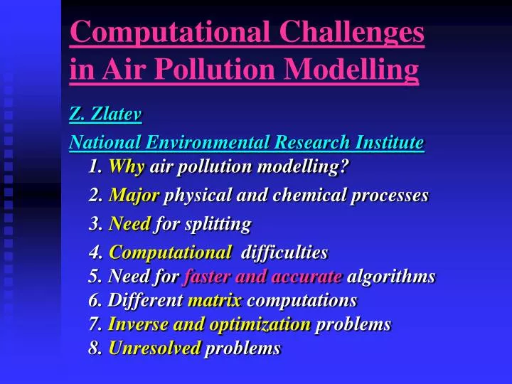
Computational Challenges in Air Pollution Modelling. Z. Zlatev National Environmental Research Institute 1. Why air pollution modelling? 2. Major physical and chemical processes 3. Need for splitting

E N D
Computational Challengesin Air Pollution Modelling Z. Zlatev National Environmental Research Institute1. Why air pollution modelling? 2. Major physical and chemical processes 3. Need for splitting 4. Computational difficulties5. Need for faster and accurate algorithms6. Different matrix computations7. Inverse and optimization problems8. Unresolved problems
1. Why air pollution models? • Distribution of the air pollution levels • Trends in the development of air pollution levels • Establishment of relationships between air pollution levels and key parameters (emissions, meteorological conditions, boundary conditions, etc.). • Predicting appearance of high levels
2. Major physical processes • Horizontal transport (advection) • Horizontal diffusion • Deposition (dry and wet) • Chemical reactions + emissions • Vertical transport and diffusion -------------------------------------------- Describe these processes mathematically
4. Need for splitting • Bagrinowskii and Godunov 1957 • Strang 1968 • Marchuk 1968, 1982 • McRay, Goodin and Seinfeld 1982 • Lancer and Verwer 1999 • Dimov, Farago and Zlatev 1999 • Zlatev 1995
4. Criteria for choosing the splitting procedure • Accuracy • Efficiency • Preservation of the properties of the involved operators
6. Size of the ODE systems • (480x480x10) grid and 35 species results in ODE systems with more than 80 mill. equations (8 mill. in the 2-D case). • More than 20000 time-steps are to be carried out for a run with meteorological data covering one month. • Sometimes the model has to be run over a time period of up to 10 years. • Different scenarios have to be tested.
7. Chemical sub-model • Parallel tasks The calculations at a given grid-point • Numerical methods QSSA (Hesstvedt et al., 1978) Backward Euler (Alexandrov et al., 1997) Trapezoidal Rule (Alexandrov et al., 1997) Runge-Kutta methods (Zlatev, 1981) Rosenbrock methods (Verwer et al., 1998) ---------------------------------------------------------- Criteria for choosing the numerical method?
8. Advection sub-model • Parallel tasks The calculations for a given compound • Numerical methods Pseudo-spectral discretization (Zlatev, 1984) Finite elements (Pepper et al., 1979) Finite differences (up-wind) “Positive” methods (Bott, 1989; Holm, 1994) Semi-Lagrangian algorithms (Neta, 1995) Wavelets (not tried yet)
11. Convergence of the Fourier series If f(x) is continuous and periodic and if f´(x) is piece-wise continuous, then the Fourier series of f(x) converges uniformly and absolutely to f(x). Davis (1963)
12. Accuracy of the Fourier series It can be proved (Davis, 1963) that if
14. Finite elements The application of finite elements in the advection module leads to an ODE system: Choice of method P is a constant matrix, H depends on the wind
15. Matrix Computations • Fast Fourier Transforms • Banded matrices • Tri-diagonal matrices • General sparse matrices • Dense matrices Typical feature: The matrices are not large, but these are to be handled many times in every sub-module during every time-step
16. Major requirements • Efficient performance on a single processor • Reordering of the operations ------------------------------------------------------ What about parallel tasks? “Parallel computation actually reflects the concurrent character of many applications” D. J. Evans (1990)
17. Chunks on one processor SIZEFujitsuSGIIBM SMP 1 76964 14847 10313 48 2611 121145225 9216 494 18549 19432 ---------------------------------------------------- First line: the straight-forward call of the box routine Last line: the vectorized option Second line: using 192 chunks ----------------------------------------------------------------------- Owczarz and Zlatev (2000)
18. “Non-optimized” code ModuleComp. timePercent Chemistry 16147 83.09 Advection 3013 15.51 Initialization 1 0.01 Input operations 50 0.26 Output operation 220 1.13 Total 19432 100.00 IBM SMP computer, one processor
19. Parallel runs on IBM SMP ProcessorsAdvectionChemistryTotal 1 933 4185 5225 2 478 1878 2427 4 244 1099 1405 8 144 521 799 16 62 272 424 --------------------------------------------------------- IBM “Night Hawk” (2 nodes); NSIZE=48
20. Scalability Process(288x288)(96x96)Ratio Advection 1523 63 24.6 Chemistry 2883 288 10.0 Total 6209 432 14.4 ------------------------------------------------------- IBM “Night Hawk” (2 nodes); NSIZE=48
22. Why is a good performance needed? GridComp. Time (96x96) 424 (45.8) (288x288) 6209 ( 3.1) Non-optimized code:19432 -------------------------------------------------------- IBM “Night Hawk” (2 nodes); NSIZE=48
23. PLANS FOR FUTURE WORK • Improving the spatial resolution of the model used to obtain information. • Object-oriented code • Predicting occurrences where the critical levels will be exceeded. • Evaluating the losses due to long exposures to high pollution levels. • Findingoptimal solutions.
24. Unresolved problems • 3-D models on fine grids • Local refinement of the grids • Data assimilation • Inverse problems • Optimization problems --------------------------------------------- Important for decision makers