Download
1 / 14
150 likes | 348 Vues
Discrete Uniform Distribution. The discrete uniform distribution occurs when there are a finite number (m) of equally likely outcomes possible. The pmf of a uniform discrete random variable X is: p(x) = 1 / m, where x=1,2,…,m The mean and variance of a discrete uniform random variable X are:.

E N D
Discrete Uniform Distribution • The discrete uniform distribution occurs when there are a finite number (m) of equally likely outcomes possible. The pmf of a uniform discrete random variable X is: p(x) = 1 / m, where x=1,2,…,m • The mean and variance of a discrete uniform random variable X are: • µ = (m + 1) / 2 • σ2 = (m2 - 1) / 12
Bernoulli Distribution • A random experiment with two possible outcomes that are mutually exclusive and exhaustive is called a Bernoulli Trial. • One outcome is arbitrarily labeled a “success” and the other a “failure” • p is the probability of a success • q = 1 - p is the probability of a failure • The Bernoulli random variable X assigns: • X(failure) = 0 and X(success) = 1
Bernoulli Distribution • The pmf for a Bernoulli random variable X is: p(x) = px (1-p)1-x, where x=0,1 • The mean and variance of a Bernoulli random variable X are: • µ = p • σ2 = pq
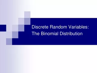
Binomial Distribution • A binomial experiment results from a sequence of n independent Bernoulli trials. • The probability of success (p) remains constant in a binomial experiment • The number of successes (X) is the random variable of interest in a binomial experiment • If Y1, Y2, …, Yn are independent Bernoulli random variables, then X=∑ Yi is a binomial random variable.
Binomial Distribution • The pmf for a Binomial random variable X is: p(x) = nCx px (1-p)n-x, where x=0,1,…,n • The mean and variance of a binomial random variable X are: • µ = np • σ2 = npq
Hypergeometric Distribution • The hypergeometric distribution applies when sampling without replacement from two possible mutually exclusive and exhaustive outcomes. • Let X be the number of objects of type 1 drawn if n objects are drawn from N where there are M objects of type 1 and N-M objects of type 2. Then X is a hypergeometric random variable and the pmf of X is:
Hypergeometric Distribution • The mean and variance of a hypergeometric random variable X are: • µ = n · (M/N) • σ2 = n · (M/N) · (1-M/N) · (N-n)/(N-1) • As M and N converge to infinity and (M/N) converges to p, the hypergeometric distribution with n samples converges to the binomial distribution with n trials and p=M/N.
Geometric Distribution • A geometric distribution occurs when sampling independent Bernoulli trials. If X is the number of Bernoulli trials until the first success is observed, then X is a geometric random variable with pmf: p(x) = (1-p)x-1p, where x=1,2,3,… • The mean and variance of a geometric random variable X are: • µ = 1 / p • σ2 = q / p2
Geometric Distribution • Notice that for integer k, P( X > k ) = qk P( X ≤ k ) = 1 – qk • “Memoryless” or “No Memory” Property • If X is a geometric random variable, then P( X > j + k | X > j ) = P( X > k ) • This implies that in independent Bernoulli trails, there is no such thing as being “due” to observe a success.
Negative Binomial Distribution • A negative binomial distribution occurs when sampling independent Bernoulli trials. If X is the number of Bernoulli trials until the rth success is observed, then X is a negative binomial random variable with pmf: p(x) = x-1Cr-1 pr (1-p)x-r, where x=r,r+1,r+2,… • The mean and variance of a negative binomial random variable X are: • µ = r (1/p) • σ2 = r (q / p2)
Poisson Distribution • The Poisson distribution describes the number of occurrences of an event in a given time or on a given interval. • Assumptions of a Poisson Process • The number of events occurring in non-overlapping intervals is independent. • The probability of 1 event occurring in a significantly short interval h is lh. • The probability of 2 events occurring in a significantly short interval h is essentially zero.
Poisson Distribution • If X is defined to be the number of occurrences of an event in a given continuous interval and is associated with a Poisson process with parameter l>0, then X has a Poisson distribution with pdf: • The mean and variance of a Poisson random variable X are: • µ = s2 = l
Poisson Distribution • If events of a Poisson process occur at a mean rate of l per unit, then the expected number of occurrences in an interval of length t is lt. Moreover, if Y is the number of occurrences in an interval of length t, it is Poisson with pdf:
Poisson Distribution • The Poisson distribution with parameter l=np is useful for approximating the binomial distribution with sample size n and probability of success p in cases with sufficiently large sample size (n>20 and p<0.05). • B(n,p) P(l=np) as n ∞, p 0, and np l