Download

1 / 13
130 likes | 276 Vues
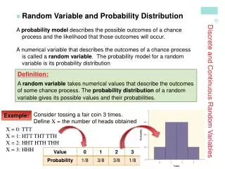
Discrete and Continuous Distribution. 01/11/2010. Hypergeometric Distribution. There are many experiments in which the condition of independence is violated and the probability of success does not remain constant for all trials. Such experiments are called hypergeometric experiments.

E N D
Discrete and Continuous Distribution 01/11/2010
Hypergeometric Distribution There are many experiments in which the condition of independence is violated and the probability of success does not remain constant for all trials. Such experiments are called hypergeometric experiments.
In other words, a hypergeometric experiment has the following properties: i) The outcomes of each trial may be classified into one of two categories, success and failure. ii) The probability of success changes on each trial. iii)The successive trials are not independent. iv)The experiment is repeated a fixed number of times.
The number of success, X in a hypergeometric experiment is called a hypergeometric random variable and its probability distribution is called thehypergeometricdistribution.
When the hypergeometric random variable X assumes a value x, the hypergeometric probability distribution is given by the formula
where N = number of units in the population, n = number of units in the sample, and k = number of successes in the population.
The hypergeometric probability distribution is appropriate when • a random sample of size n is drawn WITHOUT REPLACEMENT from a finite population of N units; ii) k of the units are of one kind (classified as success) and the remaining N – k of another kind (classified as failure).
Poisson Distribution The Poisson distribution is named after the French mathematician Sime’on Denis Poisson (1781-1840) who published its derivation in the year 1837.
The POISSON DISTRIBUTION arises in the following two situations: a) It is a limiting approximation to the binomial distribution, when p, the probability of success is very small but n, the number of trials is so large that the product np = is of a moderate size;
b) a distribution in its own right by considering a POISSON PROCESS where events occur randomly over a specified interval of time or space or length.
Such random events might be the number of typing errors per page in a book, the number of traffic accidents in a particular city in a 24-hour period, etc.
With regard to the first situation, if we assume that n goes to infinity and p approaches zero in such a way that = np remains constant, then the limiting form of the binomial probability distribution is
The Poisson distribution has only one parameter > 0. The parameter may be interpreted as the mean of the distribution.