Download
1 / 88
890 likes | 1.01k Vues
Climate Sensitivity: Linear Perspectives Isaac Held, Jerusalem, Jan 2009. 1. How can the response of such a complex system be “linear”?. Infrared radiation escaping to space - - 50km model under development at GFDL. 2.

E N D
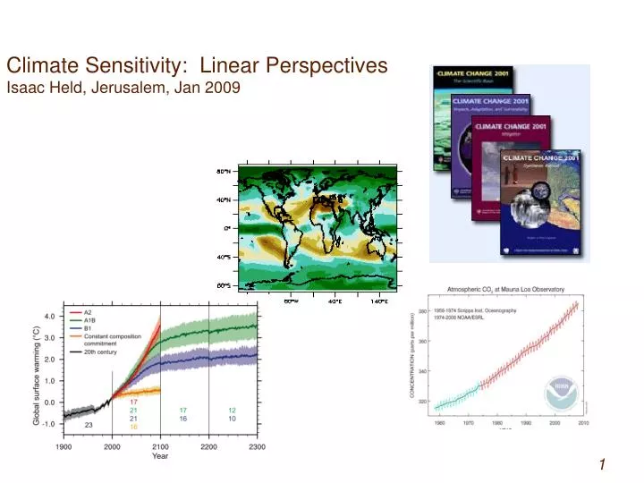
Climate Sensitivity: Linear Perspectives Isaac Held, Jerusalem, Jan 2009 1
How can the response of such a complex system be “linear”? Infrared radiation escaping to space - - 50km model under development at GFDL 2
Response of global mean temperature to increasing CO2 seems simple, as one might expect from the simplest linear energy balance models 3
But we are not interested in global mean temperature, but rather things like the response in local precipitation Percentage change in precipitation by end of 21st century: PCMDI-AR4 archive White areas => less than two thirds of the models agree on the sign of the change 4
Precipitation and evaporation “Aqua_planet” climate model (no seasons, no land surface) Instantaneous precip (lat,lon) 4a Time means
Saturation vapor pressure • 7% increase per 1K warming 20% increase for 3K 4c
GCMs match observed trend and interannual variations of tropical mean (ocean only) column water vapor when given the observed ocean temperatures as boundary condition Courtesy of Brian Soden 4d
Local vertically integrated atmospheric moisture budget: vertically integrated moisture flux precipitation vapor mixing ratio evaporation 4e
But response of global mean temperature is correlated (across GCMs) with the response of the poleward moisture flux responsible for the pattern of subtropical decrease and subpolar increase in precipitation PCMDI/CMIP3 % increase in poleward moisture flux In midlatitudes Global mean T 4f
One can see effects of poleward shift of midlatitude circulation And increase(!) in strength of Hadley cell 4g
PCMDI -AR4 Archive % Precipitation change Temperature change 5
One often sees the statement that • “Global mean is useful because averaging reduces noise” • But one can reduce noise a lot more • by projecting temperature change onto a pattern that looks like • this (pattern predicted in response to increase in CO2) • or this (observed linear trend) 6 Or one can find the pattern that maximizes the ratio of decadal scale to interannual variability – Schneider and Held 2001
“The global mean surface temperature has an especially simple relationship with the global mean TOA energy balance” ?? Seasonal OLR vs Surface T at different latitudes Seasonal OLR vs 500mb T at different latitudes Most general linear OLR-surfaceT relation 7 Relation between global means depends on spatial structure
Efficacy (Hansen et al, 2005) : Different sources of radiative forcing that provide the same net global flux at the top-of-atmosphere can give different global mean surface temperature responses Forcing for doubling CO2 roughly 3.7 W/m2 If global mean response to doubling CO2 is T2X E = efficacy = (<T> /T2X)(3.7/F) One explanation for efficacy: Responses to different forcings have different spatial structures Tropically dominated responses => E <1 Polar dominated responses => E>1 8
Why focus on top of atmosphere energy budget rather than surface? Because surface is strongly coupled to atmosphere by non-radiative fluxes (particularly evaporation) Classic example: adding absorbing aerosol does not change T, but reduces evaporation 9
If net solar flux does not change, outgoing IR does not change either (in equilibrium), -- with increased CO2, atmosphere is more opaque to infrared photons => average level of emission to space moves upwards, maintaining same T => warming of surface, given the lapse rate Final response depends on how other absorbers/reflectors (esp. clouds, water vapor, surface snow and ice) change in response to warming due to CO2, and on how the mean lapse rate changes 10
Equilibrium climate sensitivity: Double the CO2 and wait for the system to equilibrate But what is the “system”? glaciers? “natural” vegetation? Why not specify emissions rather than concentrations? Transient climate sensitivity: Increase CO2 1%/yr and examine climate at the time of doubling Typical setup – increase till doubling – then hold constant CO2 forcing ~3.7 T response W/m2 t Heat uptake by deep ocean After CO2 stabilized, warming of near surface can be thought of as due to reduction in heat uptake 11
“Observational constraints” on climate sensitivity (equilibrium or transient) Simulates some observed phenomenon: comparison with simulation constrains a,b,c … Model (a,b,c,…) predicts climate sensitivity; depends on a,b,c,… Model can be GCM – in which case constraint can be rather indirect (constraining processes of special relevance to climate sensitivity) Or it can be simple model in which climate sensitivity is determined by 1 or 2 parameters. 12
A great example of an observational constraint: looking across GCMs, strength of snow albedo feedback very well correlated with magnitude of mean seasonal cycle of surface albedos over land => observations of seasonal cycle constrain strength of feedback Hall and Xu, 2006 Can we do this for cloud feedbacks? 13
The simplest linear model forcing Heat uptake The left-hand side of this equation (the ocean model) is easy to criticize, but what about the right hand side? 14
The simplest linear model If correct, evolution should be along the diagonal N/F T/TEQ 15
Evolution in a particular GCM (GFDL’s CM2.1) for 1/% till doubling + stabilization N/F T/TEQ 16
N/F 17 EN=2 T/TEQ The efficacy of heat uptake >1 since it primarily affects subpolar latitudes Transient sensitivity affected by efficacy as well as magnitude of heat uptake
Are some of our difficulties in relating different observational constraints on sensitivity due to inadequate simple models/concepts? 18 Lots of papers, and IPCC, use concept of “Effective climate sensitivity” to estimate equilibrium sensitivity -- can’t integrate models long enough to get to accurate new equilibrium, N/F Linearly extrapolating from zero, through time of doubling, to estimate equilibrium sensitivity T/TEQ Result is time-dependent
AR4 models 2.5 2 Transient sensitivity 1.5 1 2 3 4 5 Equilibrium sensiivity Not well correlated across models – equiilbrium response brings into play feedbacks/dynamics in subpolar oceans that are surpressed in transient response 19
Response of global mean temperature in CM2.1 to instantaneous doubling of CO2 Equilibrium sensitivity >3K Transient response ~1.6K Slow response evident only after ~100 yrs and seems irrelevant for transient sensitivity Fast response 20
feedbacks T T F tropopause In equilibrium: atmosphere ocean 21
Global mean feedback analysis for CM2.1 (in A1B scenario over 21st century) base Wm-2K-1 Lapse rate total Snow/ Ice clouds Positive feedback Water vapor net “feedback” Base in isolation would give sensitivity of ~1.2K Feedbacks convert this to ~3K 22
Assorted estimates of equilibrium sensitivity Knutti+Hegerl, 2008 23
Gaussian distribution of f => skewed distribution of 1/(1-f) 25 Roe-Baker
Rough feedback analysis for AR4 models “Cloud forcing” Positive feedback 26 Cloud feedback by adjusting cloud forcing for masking effects Cloud feedback as residual Lapse rate cancels water vapor in part and reduces spread
Cloud feedback is different from change in cloud forcing 0 Cloud feedback Water vapor feedback Cloud forcing 27
Another problem A = control B = perturbation 28 Simple substitution but taking clouds from A and water vapor from B decorrelates them Soden et al, J.Clim, 2008 describe alternative ways of Alleviating this problem Not a perturbation quantity Right answer
Mostly comes from upper tropical troposphere, so negatively correlated with lapse rate feedback Annual, zonal mean water vapor kernel, normalized to correspond to % change in RH Total Clear sky 29 Difference between total and clear sky kernels used to adjust for masking effects and compute cloud feedback from change in cloud forcing
LW feedbacks positive (FAT hypothesis? => Dennis’s lecture) SW feedbacks positive/negative, and correlated with total SW and LW cloud feedback 30 Net cloud feedback from 1%/ yr CMIP3/AR4 simulations Courtesy of B. Soden
base Wm-2K-1 Lapse rate total Snow/ Ice clouds Water vapor net “feedback” 31
Weak negative “lapse rate feedback” Very strong negative “free tropospheric feedback” alternative choices of starting point (not recommended) 32 Choice of “base” = “no feedback” is arbitrary!
base Lapse rate Water vapor 33 rh What if we choose constant relative humidity rather than constant specific humidity as the base Water vapor Lapse rate Fixed rh Water vapor uniform T, fixed rh
Fixed rh uniform T base total fixed rh lapse rate Wm-2K-1 rh Snow/ ice Net “feedback” clouds 34
3.3 Non-dimensional version Clouds look like they have increased in importance (since water vapor change due to temperature change resulting from cloud change is now charged to the “ cloud” account} 1.85 clouds total Net feedback 35
Observational constraints • 20th century warming • 1000yr record • Ice ages – LGM • Deep time • Volcanoes • Solar cycle • Internal Fluctuations • Seasonal cycle etc 36
Pliocene – could our models be this wrong on the latitudinal structure ? 21st century Warming IPCC Pliocene reconstruction 37
“We conclude that a climate sensitivity greater than 1.5 6C has probably been a robust feature of the Earth’s climate system over the past 420 million years …” Royer, Berner, Park; Nature 2007 CO2 thought to be major driver of deep-time temperature variations 38 www.globalwarmingart.com
39 www.globalwarmingart.com
Global mean cooling due to Pinatubo volcanic eruption Observations with El Nino removed Range of ~10 Model Simulations GFDL CM2.1 Courtesy of G Stenchikov 40 Relaxation time after abrupt cooling contains information on climate sensitivity
Low sensitivity model Pinatubo simulation High sensitivity model Yokohata, et al, 2005 41
Observed total solar irradiance variations in 11yr solar cycle (~ 0.2% peak-to-peak) 42
Tung et al => 0.2K peak to peak (other studies yield only 0.1K) Seems to imply large transient sensitivity 4 yr damping time Only gives 0.05 peak to peak 1.8K (transient) sensitivity 43