Download
1 / 44
510 likes | 2.55k Vues
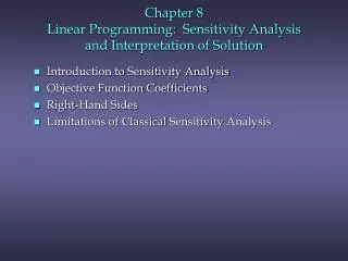
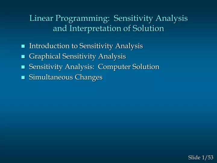
Linear Programming: Sensitivity Analysis and Interpretation of Solution. Introduction to Sensitivity Analysis Graphical Sensitivity Analysis Sensitivity Analysis: Computer Solution Simultaneous Changes. Standard Computer Output. Software packages such as TORA, LINDO and

E N D
Linear Programming: Sensitivity Analysis and Interpretation of Solution • Introduction to Sensitivity Analysis • Graphical Sensitivity Analysis • Sensitivity Analysis: Computer Solution • Simultaneous Changes
Standard Computer Output Software packages such as TORA, LINDO and Microsoft Excel Solver provide the following LP information: • Information about the objective function: • its optimal value • coefficient ranges (ranges of optimality) • Information about the decision variables: • their optimal values • their reduced costs • Information about the constraints: • the amount of slack or surplus • the dual prices • right-hand side ranges (ranges of feasibility)
Standard Computer Output Here we will discuss: • changes in the coefficients of the objective function • changes in the right-hand side value of a constraint
Sensitivity Analysis • Sensitivity analysis (or post-optimality analysis) is used to determine how the optimal solution is affected by changes, within specified ranges, in: • the objective function coefficients • the right-hand side (RHS) values • Sensitivity analysis is important to the manager who must operate in a dynamic environment with imprecise estimates of the coefficients. • Sensitivity analysis allows manager to ask certain what-ifquestions about the problem.
Example • LP Formulation Max 5x1 + 7x2 s.t. x1< 6 2x1 + 3x2< 19 x1 + x2< 8 x1, x2> 0
Example • Graphical Solution x2 x1 + x2< 8 8 7 6 5 4 3 2 1 1 2 3 4 5 6 7 8 9 10 Max 5x1 + 7x2 x1< 6 Optimal: x1 = 5, x2 = 3, z = 46 2x1 + 3x2< 19 x1
Objective Function Coefficients • Let us consider how changes in the objective function coefficients might affect the optimal solution. • The range of optimality for each coefficient provides the range of values over which the current solution will remain optimal. • Managers should focus on those objective coefficients that have a narrow range of optimality and coefficients near the endpoints of the range.
Example • Changing Slope of Objective Function x2 8 7 6 5 4 3 2 1 1 2 3 4 5 6 7 8 9 10 5 Feasible Region 4 3 1 2 x1
Range of Optimality • Graphically, the limits of a range of optimality are found by changing the slope of the objective function line within the limits of the slopes of the binding constraint lines. • The slope of an objective function line, Max c1x1 + c2x2, is -c1/c2, and the slope of a constraint, a1x1 + a2x2 = b, is -a1/a2.
Example • Range of Optimality for c1 The slope of the objective function line is -c1/c2. The slope of the first binding constraint, x1 + x2 = 8, is -1 and the slope of the second binding constraint, 2x1 + 3x2 = 19, is -2/3. Find the range of values for c1 (with c2 staying 7) such that the objective function line slope lies between that of the two binding constraints: -1 < -c1/7 < -2/3 Multiplying through by -7 (and reversing the inequalities): 14/3 <c1< 7
Example • Range of Optimality for c2 Find the range of values for c2 ( with c1 staying 5) such that the objective function line slope lies between that of the two binding constraints: -1 < -5/c2< -2/3 Multiplying by -1: 1 > 5/c2> 2/3 Inverting, 1 <c2/5 < 3/2 Multiplying by 5: 5 <c2< 15/2
Example • Range of Optimality for c1 and c2 Adjustable Cells Final Reduced Objective Allowable Allowable Cell Name Value Cost Coefficient Increase Decrease $B$8 X1 5.0 0.0 5 2 0.33333333 $C$8 X2 3.0 0.0 7 0.5 2 Constraints Final Shadow Constraint Allowable Allowable Cell Name Value Price R.H. Side Increase Decrease $B$13 #1 5 0 6 1E+30 1 $B$14 #2 19 2 19 5 1 $B$15 #3 8 1 8 0.33333333 1.66666667
Right-Hand Sides • Let us consider how a change in the right-hand side for a constraint might affect the feasible region and perhaps cause a change in the optimal solution. • The improvement in the value of the optimal solution per unit increase in the right-hand side is called the dual price. • The range of feasibility is the range over which the dual price is applicable. • As the RHS increases, other constraints will become binding and limit the change in the value of the objective function.
Dual Price • Graphically, a dual price is determined by adding +1 to the right hand side value in question and then resolving for the optimal solution in terms of the same two binding constraints. • The dual price is equal to the difference in the values of the objective functions between the new and original problems. • The dual price for a nonbinding constraint is 0. • A negative dual price indicates that the objective function will not improve if the RHS is increased.
Example • Dual Prices Constraint 1: Since x1< 6 is not a binding constraint, its dual price is 0. Constraint 2: Change the RHS value of the second constraint to 20 and resolve for the optimal point determined by the last two constraints: 2x1 + 3x2 = 20 and x1 + x2 = 8. The solution is x1 = 4, x2 = 4, z = 48. Hence, the dual price = znew - zold = 48 - 46 = 2.
Example • Dual Prices Constraint 3: Change the RHS value of the third constraint to 9 and resolve for the optimal point determined by the last two constraints: 2x1 + 3x2 = 19 and x1 + x2 = 9. The solution is: x1 = 8, x2 = 1, z = 47. The dual price is znew - zold = 47 - 46 = 1.
Example • Dual Prices Adjustable Cells Final Reduced Objective Allowable Allowable Cell Name Value Cost Coefficient Increase Decrease $B$8 X1 5.0 0.0 5 2 0.33333333 $C$8 X2 3.0 0.0 7 0.5 2 Constraints Final Shadow Constraint Allowable Allowable Cell Name Value Price R.H. Side Increase Decrease $B$13 #1 5 0 6 1E+30 1 $B$14 #2 19 2 19 5 1 $B$15 #3 8 1 8 0.33333333 1.66666667
Range of Feasibility • The range of feasibility for a change in the right hand side value is the range of values for this coefficient in which the original dual price remains constant. • Graphically, the range of feasibility is determined by finding the values of a right hand side coefficient such that the same two lines that determined the original optimal solution continue to determine the optimal solution for the problem.
Example • Range of Feasibility Adjustable Cells Final Reduced Objective Allowable Allowable Cell Name Value Cost Coefficient Increase Decrease $B$8 X1 5.0 0.0 5 2 0.33333333 $C$8 X2 3.0 0.0 7 0.5 2 Constraints Final Shadow Constraint Allowable Allowable Cell Name Value Price R.H. Side Increase Decrease $B$13 #1 5 0 6 1E+30 1 $B$14 #2 19 2 19 5 1 $B$15 #3 8 1 8 0.33333333 1.66666667
Olympic Bike Co. Olympic Bike is introducing two new lightweight bicycle frames, the Deluxe and the Professional, to be made from special aluminum and steel alloys. The anticipated unit profits are $10 for the Deluxe and $15 for the Professional. The number of pounds of each alloy needed per frame is summarized on the next slide.
Olympic Bike Co. A supplier delivers 100 pounds of the aluminum alloy and 80 pounds of the steel alloy weekly. Aluminum AlloySteel Alloy Deluxe 2 3 Professional 4 2 How many Deluxe and Professional frames should Olympic produce each week?
Olympic Bike Co. • Model Formulation • Verbal Statement of the Objective Function Maximize total weekly profit. • Verbal Statement of the Constraints Total weekly usage of aluminum alloy < 100 pounds. Total weekly usage of steel alloy < 80 pounds. • Definition of the Decision Variables x1 = number of Deluxe frames produced weekly. x2 = number of Professional frames produced weekly.
Olympic Bike Co. • Model Formulation (continued) Max 10x1 + 15x2 (Total Weekly Profit) s.t. 2x1 + 4x2 < 100 (Aluminum Available) 3x1 + 2x2 < 80 (Steel Available) x1, x2 > 0
Olympic Bike Co. • Final Solution
Olympic Bike Co. • Optimal Solution According to the output: x1 (Deluxe frames) = 15 x2 (Professional frames) = 17.5 Objective function value = $412.50
Olympic Bike Co. • Range of Optimality Question Suppose the profit on deluxe frames is increased to $20. Is the above solution still optimal? What is the value of the objective function when this unit profit is increased to $20?
Olympic Bike Co. • Sensitivity Report
Olympic Bike Co. • Range of Optimality Answer The output states that the solution remains optimal as long as the objective function coefficient of x1 is between 7.5 and 22.5. Since 20 is within this range, the optimal solution will not change. The optimal profit will change: 20x1 + 15x2 = 20(15) + 15(17.5) = $562.50.
Olympic Bike Co. • Range of Optimality Question If the unit profit on deluxe frames were $6 instead of $10, would the optimal solution change?
Olympic Bike Co. • Range of Optimality
Olympic Bike Co. • Range of Optimality Answer The output states that the solution remains optimal as long as the objective function coefficient of x1 is between 7.5 and 22.5. Since 6 is outside this range, the optimal solution would change.
Range of Optimality and 100% Rule • The 100% rule states that simultaneous changes in objective function coefficients will not change the optimal solution as long as the sum of the percentages of the change divided by the corresponding maximum allowable change in the range of optimality for each coefficient does not exceed 100%.
Olympic Bike Co. • Range of Optimality and 100% Rule Question If simultaneously the profit on Deluxe frames was raised to $16 and the profit on Professional frames was raised to $17, would the current solution be optimal?
Olympic Bike Co. • Range of Optimality and 100% Rule Answer If c1 = 16, the amount c1 changed is 16 - 10 = 6 . The maximum allowable increase is 22.5 - 10 = 12.5, so this is a 6/12.5 = 48% change. If c2 = 17, the amount that c2 changed is 17 - 15 = 2. The maximum allowable increase is 20 - 15 = 5 so this is a 2/5 = 40% change. The sum of the change percentages is 88%. Since this does not exceed 100%, the optimal solution would not change.
Range of Feasibility and 100% Rule • The 100% rule states that simultaneous changes in right-hand sides will not change the dual prices as long as the sum of the percentages of the changes divided by the corresponding maximum allowable change in the range of feasibility for each right-hand side does not exceed 100%.
Olympic Bike Co. • Range of Feasibility Question What is the maximum amount the company should pay for 50 extra pounds of aluminum?
Olympic Bike Co. • Range of Feasibility
Olympic Bike Co. • Range of Feasibility Answer The shadow price provides the value of extra aluminum. The shadow price for aluminum is the same as its dual price (for a maximization problem). The shadow price for aluminum is $3.125 per pound and the maximum allowable increase is 60 pounds. Because 50 is in this range, the $3.125 is valid. Thus, the value of 50 additional pounds is = 50($3.125) = $156.25.
Example 3 • Consider the following linear program: Min 6x1 + 9x2 ($ cost) s.t. x1 + 2x2 < 8 10x1 + 7x2 > 30 x2 > 2 x1, x2> 0
Example 3 • Range of Optimality Question Suppose the unit cost of x1 is decreased to $4. Is the current solution still optimal? What is the value of the objective function when this unit cost is decreased to $4?
Example 3 • Range of Optimality Question How much can the unit cost of x2 be decreased without concern for the optimal solution changing?
Example 3 • Range of Optimality and 100% Rule Question If simultaneously the cost of x1 was raised to $7.5 and the cost of x2 was reduced to $6, would the current solution remain optimal?
Example 3 • Range of Feasibility Question If the right-hand side of constraint 3 is increased by 1, what will be the effect on the optimal solution?