Download
1 / 34
340 likes | 412 Vues
Random Variables. : 9 10 11 12. Numerical Outcomes. Consider associating a numerical value with each sample point in a sample space. (1,1) (1,2) (1,3) (1,4) (1,5) (1,6) (2,1) (2,2) (2,3) (2,4) (2,5) (2,6) (3,1) (3,2) (3,3) (3,4) (3,5) (3,6)

E N D
:9101112 Numerical Outcomes • Consider associating a numerical value with each sample point in a sample space. • (1,1) (1,2) (1,3) (1,4) (1,5) (1,6) • (2,1) (2,2) (2,3) (2,4) (2,5) (2,6) • (3,1) (3,2) (3,3) (3,4) (3,5) (3,6) • (4,1) (4,2) (4,3) (4,4) (4,5) (4,6) • (5,1) (5,2) (5,3) (5,4) (5,5) (5,6)(6,1) (6,2) (6,3) (6,4) (6,5) (6,6) • The function relating each outcome from a roll of the die with their sum is considered a random variable. • Refer to values of the random variable as events. For example, {Y = 9}, {Y = 10}, etc.
Probability Y = y • The probability of an event, such as {Y = 9} is denoted P(Y = 9). • In general, for a real number y, the probability of {Y = y} is denoted P(Y = y), or simply, p( y). • P(Y = 10) or p(10) is the sum of probabilities for sample points which are assigned the value 10. • When rolling two dice, P(Y = 10) = P({(4, 6)}) + P({(5, 5)}) + P({(6, 4)}) = 1/36 + 1/36 + 1/36 = 3/36
Discrete Random Variable • A discrete random variable is a random variable that only assumes a finite (or countably infinite) number of distinct values. • For an experiment whose sample points are associated with the integers or a subset of integers, the random variable is discrete.
Probability Distribution • A probability distribution describes the probability for each value of the random variable. y p(y)2 1/363 2/364 3/365 4/366 5/367 6/368 5/369 4/3610 3/3611 2/3612 1/36 Presented as a table, formula, or graph.
Probability Distribution • For a probability distribution: y p(y)2 1/363 2/364 3/365 4/366 5/367 6/368 5/369 4/3610 3/3611 2/3612 1/36 = 1.0 Here we may take the sum just over those values of yfor which p(y) is non-zero.
Expected Value • The “long run theoretical average” • For a discrete R.V. with probability function p(y), define the expected value of Y as: • In a statistical context, E(Y) is referred to as the mean and so E(Y) and m are interchangeable.
For a constant multiple… • Of course, a constant multiple may be factored out of the sum • Thus, for our circles, E(C) = E(2pR) = 2pE(R).
For a constant function… • In particular, if g(y) = c for all y in Y, then E[g(Y)] = E(c) = c.
Function of a Random Variable • Suppose g(Y) is a real-valued function of a discrete random variable Y. It follows g(Y) is also a random variable with expected value • In particular, for g(Y) = Y2, we have
Try this! • For the following distribution: • Compute the values E( Y ), E( 3Y ), E( Y2 ), and E( Y3 )
For sums of variables… • Also, if g1(Y) and g2(Y) are both functions of the random variable Y, then
All together now… • So, when working with expected values, we have • Thus, for a linear combination Z = c g(Y) + b,where c and b are constants:
Try this! • For the following distribution: • Compute the values E( Y2 + 2 ), E( 2Y+ 5 ), and E( Y2 - Y)
Variance, V(Y) • For a discrete R.V. with probability function p(y), define the variance of Y as: • Here, we use V(Y) and s2 interchangeably to denote the variance. The positive square root of the variance is the standard deviation of Y. • It can be shown that • Note the variance of a constant is zero.
Computing V(Y) • And applying our rules for expected value, we find variance may be expressed as (as the mean is a constant) When computing the variance, it is often easier to use the formula
Try this! • For the following distribution: • Compute the values V(Y) , V(2Y), and V(2Y + 5). • How would you compute V(Y2) ?
“Moments and Mass” • Note the probability function p(y) for a discrete random variable is also called a “probability mass” or “probability density” function. • The expected values E(Y) and E(Y2) are called the first and second moments, respectively.
Continuous Random Variables • For discrete random variables, we required that Y was limited to a finite (or countably infinite) set of values. • Now, for continuous random variables, we allow Y to take on any value in some interval of real numbers. • As a result, P(Y = y) = 0 for any given value y.
CDF • For continuous random variables, define the cumulative distribution functionF(y) such that Thus, we have
PDF • For the continuous random variable Y, define the probability density function as for each y for which the derivative exists.
Integrating a PDF • Based on the probability density function,we may write Remember the 2nd Fundamental Theorem of Calc.?
Properties of a PDF • For a density function f(y): • 1).f(y) > 0 for any value of y. • 2). Density function, f(y) Distribution function, F(y)
Try this! • For what value of k is the following function a density function? • We must satisfy the property
Try this! • For what value of k is the following function a density function? • Again, we must satisfy the property
P(a < Y < b) • To compute the probability of the eventa < Y < b ( or equivalently a< Y <b ),we just integrate the PDF:
Try this! • For the previous density function • Find the probability • Find the probability
Try this! • Suppose Y is time to failure and • Determine the density function f (y) • Find the probability • Find the probability
Expected Value, E(Y) • For a continuous random variable Y, define the expected value of Y as • Note this parallels our earlier definition for the discrete random variable:
Expected Value, E[g(Y)] • For a continuous random variable Y, define the expected value of a function of Y as • Again, this parallels our earlier definition for the discrete case:
Properties of Expected Value • In the continuous case, all of our earlier properties for working with expected value are still valid.
Properties of Variance • In the continuous case, our earlier properties for variance also remain valid. and
Problem from MAT 332 • Find the mean and variance of Y, given