Download
1 / 27
280 likes | 463 Vues
Random Variables. Section 3.1. A Random Variable: is a function on the outcomes of an experiment; i.e. a function on outcomes in S . For discrete random variables , we call P ( X = x ) = P ( x ) the probability mass function ( pmf ) . .

E N D
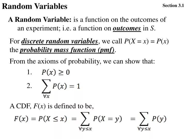
Random Variables Section 3.1 A Random Variable: is a function on the outcomes of an experiment; i.e. a function on outcomes in S. For discrete random variables, we call P(X = x) = P(x) the probability mass function (pmf). From the axioms of probability, we can show that: 1. 2. A CDF, F(x) is defined to be,
Expected values Section 3.3 The expected value E(X) of a discrete random variable is the weighted average or the mean of that random variable, The variance of a discrete random variable is the weighted average of the squared distance from the mean, The standard deviation, Let h(X) be a function, a and b be constants then,
The Binomial Distribution Section 3.4 An experiment is called a binomial experiment if it satisfies the following conditions: The experiment of interest here consists of a sequence of n sub-experiments called trials, where n is fixed in advance of the experiment. Each trial can result in one of two outcomes usually denoted by success (S) or failure (F). These trials are independent (outcome of one trial doesn’t affect any of the others). The probability of success, p, is constant from trial to trial
The Binomial Distribution Section 3.4 What the above is saying: The experiment consists of a group of nindependent Bernoulli sub-experiments, where n is fixed in advance of the experiment and the probability of a success is p. What we are interested in studying is the number of successes that we may observe in any run of such an experiment.
The Binomial Distribution Section 3.4 Example: Each component of the following system (components connected in parallel) has a 0.1 chance of breaking down (crazy enough is called a success). Assuming that none of these components affect the performance of any of the others, construct the associated probability distribution. 0.1 0.1 0.1 0.1 0.1
The Binomial Distribution Section 3.4 As we have seen in studying uncertainty: Identify the experiment of interest and understand it well (including the associated population) Identify the sample space (all possible outcomes) Identify an appropriate random variable that reflects what you are studying (and simple events based on this random variable) Construct the probability distribution associated with the simple events based on the random variable
The Binomial Distribution Section 3.4 Identify the experiment of interest and understand it well (including the associated population) A binomial experiment! The experiment consists of a group of nindependent Bernoulli sub-experiments, where n is fixed in advance of the experiment and the probability of a success is p.
The Binomial Distribution Section 3.4 Identify the sample space (all possible outcomes) S = {SSSSS, SSSSF, SSSFS, SSFSS, SFSSS, FSSSS, SSSFF, SSFSF, …, FFFFF} How many possible outcomes? All equally likely? Find the probability of one of the simple events?
The Binomial Distribution Section 3.4 Identify an appropriate random variable that reflects what you are studying (and simple events based on this random variable) What we are interested in studying in these experiments is the number of successes that we may observe in any run of the experiment. So the random variable of interest is: Snew= {0, 1, 2, 3, 4, 5}
The Binomial Distribution Section 3.4 Construct the probability distribution associated with the simple events based on the random variable X = 0 => no success! In how many different ways can we have zero success? To answer this we need to know if order maters or not! In a Binomial experiment a success is a success no matter where it happens; i.e. order doesn’t matter! Number of ways to get zero successes is? The probability of a zero success is?
The Binomial Distribution Section 3.4 Construct the probability distribution associated with the simple events based on the random variable X = 1 => one success! One of those is {SFFFF} The probability of this specific simple event is? In how many different ways can we have one success? Need to count the number of ways in which we can order 5 objects with 1 S and 4 indistinguishable F’s! So, probability of one success is?
The Binomial Distribution Section 3.4 Construct the probability distribution associated with the simple events based on the random variable X = 2 => two successes! One of those is {SSFFF} The probability of this specific simple event is? In how many different ways can we have two successes? Need to count the number of ways in which we can order 5 objects with 2 indistinguishable S’s and 3 indistinguishable F’s! So, probability of two successes is?
The Binomial Distribution Section 3.4 Construct the probability distribution associated with the simple events based on the random variable X = 3 => three successes! One of those is {SSSFF} X = 4 => four successes! One of those is {SSSSF} X = 5 => five successes! {SSSSS} So, in general for any x, P(X=x) is For any n and any x, P(X=x) is
The Binomial Distribution Section 3.4 Construct the probability distribution associated with the simple events based on the random variable The resulting distribution in table format: Found using dbinom(x, n, p) in R Can be found using the CDF given in table A.1 (which you might use in the next exam)
The Binomial Distribution Section 3.4 Notation in association with the binomial experiment: The binomial random variable X = the number of successes (S’s) among n Bernoulli trials or sub-experiments. We say X is distributed Binomial with parameters n and p,
The Binomial Distribution Section 3.4 Notation in association with the binomial experiment: The pmf can become (depending on the book), The CDF can become (also depending on the book),
The Binomial Distribution Section 3.4 The mean, the variance and the standard deviation:
The Binomial Distribution Section 3.4 When to use the binomial distribution? When we have n independent Bernoulli trials When each Bernoulli trial is formed from a sample n of individuals (parts, animals, …) from a population with replacement. When each Bernoulli trial is formed from a sample of n individuals (parts, animals, …) from a population of size Nwithout replacement if n/N < 5%.
The Binomial Distribution Section 3.4 Example: Ten light bulbs were chosen at random from a batch of 10000 produced by GE. If we know that 100 of these light bulbs are defective, what is the chance that we will observe 2 or more defectives in this sample? If we sample with replacement.
The Binomial Distribution Section 3.4 As we have seen in studying uncertainty: Identify the experiment of interest and understand it well (including the associated population) Identify the sample space (all possible outcomes) Identify an appropriate random variable that reflects what you are studying (and simple events based on this random variable) Construct the probability distribution associated with the simple events based on the random variable
The Binomial Distribution Section 3.4 Example: Ten light bulbs were chosen at random from a batch of 10000 produced by GE. If we know that 100 of these light bulbs are defective, what is the chance that we will observe 2 or more defectives in this sample? If we sample without replacement.
The Binomial Distribution Section 3.4 A touch on inference: Say that one day we passed by the factory of the first example and we found that 4 machines (out of the 5) are not working. Do you think that the model (governed by the parameters n = 5 and p = 0.1) is appropriate to describe this system? Why? Or why not? Can you find a better model (i.e. a better value of the parameters) that fits this observed data?
The Binomial Distribution Section 3.4 The resulting distribution in table format:
The Binomial Distribution Section 3.4
The Binomial Distribution Section 3.4
The Binomial Distribution Section 3.4
The Binomial Distribution Section 3.4 So this sample either happened by chance with probability 0.00045, if the model we are using is true, or is best described by a model with p = 0.8. The likelihood of this data under the current model is 0.00045 and under the new model is 0.4096 So, if the p = 0.1 is not known for sure (it usually is) then, based on our observation, we favor a model with p = 0.8. What kind of implications does this have for the factory?