Download
1 / 45
460 likes | 687 Vues
A stochastic dimension reduction for stochastic PDEs. Nicholas Zabaras. Materials Process Design and Control Laboratory Sibley School of Mechanical and Aerospace Engineering 101 Frank H. T. Rhodes Hall Cornell University Ithaca, NY 14853-3801 Email: zabaras@cornell.edu

E N D
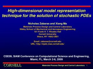
A stochastic dimension reduction for stochastic PDEs Nicholas Zabaras Materials Process Design and Control Laboratory Sibley School of Mechanical and Aerospace Engineering101 Frank H. T. Rhodes Hall Cornell University Ithaca, NY 14853-3801 Email: zabaras@cornell.edu URL: http://mpdc.mae.cornell.edu/
Outline of the presentation • Problem definition • Adaptive sparse grid collocation method (ASGC)1 • High dimensional model representation2 • Example: Flow through random heterogeneous media • Conclusions 1. X. Ma, N. Zabaras, A hierarchical adaptive sparse grid collocation method for the solution of stochastic differential equations, Journal of Computational physics, Vol. 228 , pp. 3084-3113, 2009. 2. X. Ma, N. Zabaras, A adaptive high dimensional stochastic model representation technique for the solution of stochastic differential equations, Journal of Computational physics, submitted, 2009. 2
Motivation All physical systems have inherent associated randomness • SOURCES OF UNCERTAINTIES • Multiscale nature inherently statistical • Uncertainties in process conditions • Material heterogeneity • Model formulation – approximations, • assumptions Why uncertainty modeling? Assess product and process reliability Estimate confidence level in model predictions Identify relative sources of randomness Provide robust design solutions 3
Motivation of HDMR • Conventional and adaptive collocation methods are not suitable for high-dimensional problems due to their weakly dependence on the dimensionality (logarithmic) in the error estimate. • Although ASGC can alleviate this problem to some extent, its performance depends on the regularity of the problem and the method is only effective when some random dimensions are more important than others. CSGC • In e.g. random heterogeneous media we often deal with a very small correlation length and this results in a rather high-dimensional stochastic space with nearly the same weights along each dimension. In this case, all the previously developed stochastic methods are obviously not applicable. • These modeling issues for high-dimensional stochastic problems motivate the use of the High Dimensional Model Representation (HDMR) technique. 4
Problem definition • Define a complete probability space . We are interested to find a stochastic function such that for P-almost everywhere (a.e.) , the following holds: where are the coordinates in , L is a differential operator, and B denotes boundary condition operators. • L and B as well as the driving terms f and g can be assumed random. • In general, we require an infinite number of random variables to completely characterize a stochastic process. This poses a numerical challenge in modeling uncertainty in physical quantities that have spatio-temporal variations, hence necessitating the need for a reduced-order representation. • By using e.g. the Karhunen-Loève expansion, the random input can be characterized by a set of random variables.
The finite-dimensional noise assumption • By using the Doob-Dynkin lemma, the solution of the problem can be described by the same set of random variables, i.e. • So the original problem can be restated as: Find the stochastic function such that • In this work, we assume that are independent random variables with probability density function . Let be the image of . Then is the joint probability density of with support
Stochastic collocation based framework Need to represent this function Sample the function at a finite set of points Use polynomials (Lagrange polynomials) to get a approximate representation Function value at any point is simply Stochastic function in 2 dimensions Spatial domain is approximated using a FEM discretization. Stochastic domain is approximated using multidimensional interpolating functions 8 8
Choice of collocation points and nodal basis functions • In the context of incorporating adaptivity, we use the Newton-Cotes grid with equidistant support nodes and the linear hat function as the univariate nodal basis. • In this manner, one ensures a local support and that discontinuities in the stochastic space can be resolved. The piecewise linear basis functions is defined as 9 9
Conventional sparse grid collocation (CSGC) • Denote the one dimensional interpolation formula as LET OUR BASIC 1D INTERPOLATION SCHEME BE SUMMARIZED AS • In higher dimensions, a simple case is the tensor product formula IN MULTIPLE DIMENSIONS, THIS CAN BE WRITTEN AS • Using the 1D formula, the sparse interpolant , where is the depth of sparse grid interpolation and is the number of stochastic dimensions, is given by the Smolyak algorithm as • Here, we define the hierarchical surplus as: 10
Nodal basis versus hierarchical basis Nodal basis Hierarchical basis
Hierarchical Integration • The mean of the random solution can be evaluated as follows: • Denoting we rewrite the mean as • To obtain the variance of the solution, we need to first obtain an approximate expression for 12
Adaptive sparse grid collocation (ASGC)1 Let us first revisit the 1D hierarchical interpolation • For smooth functions, the hierarchical surpluses tend to zero as the interpolation level increases. • Finite discontinuities are indicated by the magnitude of the hierarchical surplus. • The bigger the magnitude is, the stronger the underlying discontinuity is. • Therefore, the hierarchical surplus is a natural candidate for error control and adaptivity. If the hierarchical surplus is larger than a pre-defined value (threshold), we simply add the 2N neighboring points to the current point. 1 .X. Ma, N. Zabaras, An hierarchical adaptive sparse grid collocation method for the solution of stochastic differential equations, JCP, 228 (2009) 3084-3113. 13 13
Adaptive sparse grid collocation • By using the equidistant nodes, it is easy to refine the grid locally around the non-smooth region. • We consider the 1D equidistant points of the sparse grid as a tree-like data structure • Then we can consider the interpolation level of a grid point Y as the depth of the tree D(Y). For example, the level of point 0.25 is 3. • Denote the father of a grid point as F(Y), where the father of the root 0.5 is itself, i.e. F(0.5) = 0.5. • Thus the conventional sparse grid in N- dimensional random space can be reconsidered as
Adaptive sparse grid collocation • Thus, we denote the sons of a grid point by • From this definition, it is noted that, in general, for each grid point there are two sons in each dimension, therefore, for a grid point in a N- dimensional stochastic space, there are 2N sons. • The sons are also the neighbor points of the father, which are just the support nodes of the hierarchical basis functions in the next interpolation level. • By adding the neighbor points, we actually add the support nodes from the next interpolation level, i.e. we perform interpolation from level |i| to level |i|+1. • In this way, we refine the grid locally while not violating the developments of the Smolyak algorithm.
Definition of the error indicator • The mean of the random solution can be evaluated as follows: • Denoting we rewrite the mean as • We now define the error indicator as follows: • In addition to the surpluses, this error indicator incorporates information from the basis functions. This forces the error to decrease to a sufficient small value for a large interpolation level. This error indicator guarantees that the refinement would stop at a certain interpolation level.
Adaptive sparse grid interpolation Ability to detect and reconstruct steep gradients
High dimensional model representation (HDMR)1 • Let be a real-value multivariate stochastic function: , which depends on a N-dimensional random vector . A HDMR of can be described by where the interior sum is over all sets of integers , that satisfy .This relation means that It can be viewed as a finite hierarchical correlated function expansion in terms of the input random variables with increasing dimensions. • For most physical systems, the first- and second-order expansion terms are expected to have most of the impact upon the output. 1. O. F. Alis, H. Rabitz, General foundations of high dimensional representations, Journal of Mathematical Chemistry 25 (1999) 127-142. 20
High dimensional model representation (HDMR) In this expansion: • denotes the zeroth-order effect which is a constant. • The component function gives the effect of the variable acting independently of the other input variables. • The component function describes the interactive effects of the variables and . Higher-order terms reflect the cooperative effects ofincreasingnumbers of variables acting together to impact upon . • The last term gives any residual dependence of all the variables locked together in a cooperative way to influence the output . 21
HDMR: Compact notation • This equation is often written in a more compact notation: for a given set where denotes the set of coordinate indices and . Here, denotes the - dimensional vector containing those components of whose indices belong to the set , where is the cardinality of the corresponding set , i.e. . • For example, if , then and implies • The component functions can be derived by minimizing the error functional subject to the orthogonal constraint for
HDMR: Component functions • The measure determines the particular form of the error functional and of the component functions. • By the variational principle, the component functions can be explicitly given as where the measure induces the projection operator where • There are two different forms of HDMR induced by different measure: ANOVA-HDMR and CUT-HDMR.
ANOVA-HDMR versus CUT-HDMR HDMR ANOVA-HDMR CUT-HDMR Dirac measure Lebesgue measure at a reference point dimensional integration dimensional function Computational expensive -- requires a N-dimensional integral for the constant terms Computational efficient -- requires function evaluations at sample points
Therefore, the -dimensional stochastic problem is transformed to several lower-order -dimensional problems which can easily solved by ASGC: CUT-HDMR • Within the framework of CUT-HDMR, we can write where the notation means that the components of other than those indices that belong to the set equal to those of the reference point. • If the HDMR is a converged expansion, the choice of this point does not affect the approximation. In this work, the mean of the random input vector is chosen as the reference point. where are the hierarchical surpluses for different sub-problems indexed by and is only a function of the coordinates belonging to
CUT-HDMR • Let us denote as the mean of the component function . Then the mean of the HDMR expansion is simply . • The basic conjecture underlying HDMR is that the component functions arising in typical physical systems will not likely exhibit high-order cooperativity among the input variables such that the 1st- and 2nd-order expansion terms are expected to have most of the impact upon the output and the contribution of higher-order terms would be insignificant. • In other words, instead of solving the N - dimensional problem directly using ASGC, which is impractical for extremely high dimensional problems, we only need to solve several one- or two- dimensional problems, which can be solved efficiently via ASGC.
Effective dimension of a stochastic function • Let be the sum of all contributions to the mean value. Here, denotes the norm. • Then, for the proportion , the truncation dimension is defined as the smallest integer , such that whereas, the superposition dimension is defined as the smallest integer , such that • The superposition dimension is also called the order of the HDMR expansion. • With the definition of effective dimensions, we can thus truncate the expansion and take only a subset of all indices . Here we assume that the set satisfies the following admissibility condition: This is to guarantee that all the terms can be calculated via the recursive expression for computing the component functions.
Effective dimension of a stochastic function • In practice, we always truncate the expansion by taking only a subset of all indices . We can define an interpolation formula for the approximation of as • It is common to refer to the terms collectively as the l- “order- terms”. Then the expansion order is the maximum of . The number of collocation points in this expansion is defined as the sum of the number of points for each sub-problem, i.e. • However, the number of order- component functions is , which increases quickly with the number of dimensions. Therefore, we developed an adaptive version of HDMR.
Approximation error • We fix and assume that and , the corresponding superposition and truncation dimensions, are known. With the definition of the index set , we have the following theorem: • Therefore, it is expected that the expansion converges to the true value with decreasing error threshold and increasing number of component functions.
Adaptive HDMR • For extremely high dimensional problems, even a 2nd order expansion is impractical due to the increase of the number of component functions. Therefore, we would like to develop an adaptive version of HDMR for automatically and simultaneously detecting the truncation and superposition dimensions. • We assume each component function is associated with a weight which describes the contribution of the term to the HDMR. • First, we try to find the important dimensions. To this end, we always construct the 0th - and 1st-order HDMR expansion. We define a weight: Then we define the important dimensions as those whose weights are larger than a predefined error threshold . Only higher-order terms which consist of only these important dimensions are considered. Here, the norm is defined in the spatial domain.
Adaptive HDMR • For example, if the important dimensions are 1, 3 and 5, then only the higher-order terms {13}, {15}, {35} and {135} are considered. • However not all the possible terms are computed. For higher-order term, a weight is also defined as We also define the important terms in a similar way. We put all the important dimensions and higher-order terms in to a set . When adaptively constructing HDMR for each new order, we only calculate the term whose indices satisfy the admissibility relation
Adaptive HDMR • Continued with the example, now if we want to construct the 2nd -order expansion, only {13}, {15} and {35} are calculated. • Then we compute the weights for each term. Assume {13} is the important term, the important index set • Now, we go to 3rd order expansion. The only possible term is {135}. Its subsets {13} and {15} do not belong to the important index set , i.e. {1,3,5} does not satisfy the admissibility condition. Therefore, the construction stops. • In other words, among all possible indices, we only find the terms which can be computed using the previous known important component functions and have significant contributions to the overall expansion.
Adaptive HDMR • Let us denote the order of expansion as Furthermore, we also define a relative error of the integral value between two consecutive expansion orders and as • If is smaller than another predefined error threshold , the HDMR is regarded as converged and the construction stops. • In this way, the construction will automatically stop and then the obtained HDMR expansion can be used as a stochastic surrogate model (response surface) for the solution. Any statistics can be easily computed through this expansion.
production well injection well Numerical example: Flow through random media Basic equation for pressure and velocity in a domain where denotes the deterministic source/sink term. Homogeneous boundary condition is applied. Mixed finite element method is used to solve the deterministic problem at the collocation points. • To impose the non-negativity of the permeability, we will treat the permeability as a log random field obtained from the K-L expansion where is a zero mean Gaussian random field with covariance function where is the correlation length and is the standard deviation. 35
Numerical example: K-L Expansion Series of eigenvalues and their finite sums for three different correlation lengths at • The eigenvalues and their corresponding eigenfunctions can be determined analytically. The are assumed as i.i.d. uniform random variables on [-1,1]. • According to the decay rate of eigenvalues, the number of stochastic dimensions is and , respectively for and . • Monte Carlo simulations are conducted for the purpose of comparison. For each case, the reference solution is taken from samples and all errors are defined as normalized errors. In all cases, .
Standard deviation of the velocity-component along the cross section for different correlation lengths Standard deviation for different correlation lengths Number of component functions is 2271 while for the full 2nd-order expansion it is 125251. The advantage of using adaptive HDMR is obvious.
PDF of the velocity-component at point for different correlation lengths PDF at (0,0.5) for different correlation lengths
PDF at (0,0.5) for different correlation lengths • Each PDF is generated by plotting the kernel density estimate of 10000 output samples through sampling the input space and computing the output value through the HDMR approximation. • The spatial variability determines the total input variability, which further determines the interactive effects between the input variables. The larger the input variability is, the stronger the interactive effects are. The role of HDMR component functions is to capture these input effects upon the output. • The higher the input variability is, the more component functions are needed. In our case, represents a rather high input variability. Higher order terms are therefore needed to capture these effects whereas only 1st -order terms are not enough. • The computed PDFs indicate that the corresponding HDMR approximations are indeed very accurate. Therefore, we can obtain any statistic from this stochastic reduced-order model, which is an advantage over the MC method.
Convergence of the normalized errors of the standard deviation of the velocity-component for different correlation lengths Convergence of the normalized errors Algebraic convergence rate better than MC Nearly the same for three cases, it does not depend on the smoothness of the random space
Standard deviation of the velocity-component along the cross section for different . Standard deviations for different with
PDF of the velocity-component at point for different PDF at (0,0.5) for different with For low input variability, even 1st - order expansion is accurate For moderate input variability, 1st order does not deviate significantly from MC. However, a few 2nd -order terms are still needed. For high input variability, the 1st -order expansion deviates from MC. More component terms are needed to improve accuracy.
Convergence of the normalized errors of the standard deviation of the velocity-component for different Convergence of the normalized errors with Direct solution of the 500 dimensional problem using ASGC is impractical due to the huge computational cost. Convergence rate deteriorates with increasing input variability. However, it is still better than that of MC
Conclusions • An adaptive dimensional stochastic model representation technique for solving high-dimensional SPDEs is introduced. • HDMR decomposes the original N-dimensional stochastic problem into several low-dimensional sub-problems. • By combining HDMR and ASGC, high-dimensional stochastic problems can be solved accurately and efficiently. • The numerical examples show that the number of component functions needed in the HDMR for a fixed stochastic dimension depends more on the input variability than the smoothness of the random space. • This method to our knowledge is the first approach which can solve high-dimensional stochastic problems by reducing dimensions from truncation of HDMR and resolve low-regularity by local adaptivity through ASGC.
Other work on model reduction for SPDEs • Develop a stochastic (non-linear) version of POD – use random snapshots, different projection norms in stochastic space, .. • Use data-driven manifold learning approaches to reduce the dimensionality of the stochastic input while simultaneously computing the random space support and the joint distribution of the random variables. • Similar ideas can be applied to the stochastic output using simulated random system response snapshots. • Stochastic model reduction of multiscale data (bi-orthogonal decomposition as a generalization of KLE expansions, etc.)