Download
1 / 59
600 likes | 778 Vues
Multiple Access. Mahesh Jangid Assistant Professor JVW University. Figure 12.1 Data link layer divided into two functionality-oriented sublayers. Figure 12.2 Taxonomy of multiple-access protocols discussed in this chapter. 12-1 RANDOM ACCESS.

E N D
Multiple Access Mahesh Jangid Assistant Professor JVW University
Figure 12.1 Data link layer divided into two functionality-oriented sublayers
Figure 12.2 Taxonomy of multiple-access protocols discussed in this chapter
12-1 RANDOM ACCESS In random access or contention methods, no station is superior to another station and none is assigned the control over another. No station permits, or does not permit, another station to send. At each instance, a station that has data to send uses a procedure defined by the protocol to make a decision on whether or not to send. Topics discussed in this section: ALOHACarrier Sense Multiple Access Carrier Sense Multiple Access with Collision Detection Carrier Sense Multiple Access with Collision Avoidance
Example 12.2 A pure ALOHA network transmits 200-bit frames on a shared channel of 200 kbps. What is the requirement to make this frame collision-free? Solution Average frame transmission time Tfr is 200 bits/200 kbps or 1 ms. The vulnerable time is 2 × 1 ms = 2 ms. This means no station should send later than 1 ms before this station starts transmission and no station should start sending during the one 1-ms period that this station is sending.
Note The throughput for pure ALOHA is S = G × e −2G . The maximum throughput Smax = 0.184 when G= (1/2).
Example 12.3 A pure ALOHA network transmits 200-bit frames on a shared channel of 200 kbps. What is the throughput if the system (all stations together) produces a. 1000 frames per second b. 500 frames per second c. 250 frames per second. Solution The frame transmission time is 200/200 kbps or 1 ms. a. If the system creates 1000 frames per second, this is 1 frame per millisecond. The load is 1. In this case S = G× e−2 G or S = 0.135 (13.5 percent). This means that the throughput is 1000 × 0.135 = 135 frames. Only 135 frames out of 1000 will probably survive.
Example 12.3 (continued) b. If the system creates 500 frames per second, this is (1/2) frame per millisecond. The load is (1/2). In this case S = G × e −2G or S = 0.184 (18.4 percent). This means that the throughput is 500 × 0.184 = 92 and that only 92 frames out of 500 will probably survive. Note that this is the maximum throughput case, percentagewise. c. If the system creates 250 frames per second, this is (1/4) frame per millisecond. The load is (1/4). In this case S = G × e −2G or S = 0.152 (15.2 percent). This means that the throughput is 250 × 0.152 = 38. Only 38 frames out of 250 will probably survive.
Note The throughput for slotted ALOHA is S = G × e−G . The maximum throughput Smax = 0.368 when G = 1.
Example 12.4 A slotted ALOHA network transmits 200-bit frames on a shared channel of 200 kbps. What is the throughput if the system (all stations together) produces a. 1000 frames per second b. 500 frames per second c. 250 frames per second. Solution The frame transmission time is 200/200 kbps or 1 ms. a. If the system creates 1000 frames per second, this is 1 frame per millisecond. The load is 1. In this case S = G× e−G or S = 0.368 (36.8 percent). This means that the throughput is 1000 × 0.0368 = 368 frames. Only 386 frames out of 1000 will probably survive.
Example 12.4 (continued) b. If the system creates 500 frames per second, this is (1/2) frame per millisecond. The load is (1/2). In this case S = G × e−G or S = 0.303 (30.3 percent). This means that the throughput is 500 × 0.0303 = 151. Only 151 frames out of 500 will probably survive. c. If the system creates 250 frames per second, this is (1/4) frame per millisecond. The load is (1/4). In this case S = G × e −G or S = 0.195 (19.5 percent). This means that the throughput is 250 × 0.195 = 49. Only 49 frames out of 250 will probably survive.
Figure 12.10 Behavior of three persistence methods 1-persistent: • Stations having a packet to send sense the channel continuously, waiting until the channel becomes idle. • As soon as the channel is sensed idle, they transmit their packet. • If more than one station is waiting, a collision occurs. • Stations involved in a collision perform a the backoff algorithm to schedule a future time for resensing the channel • Optional backoff algorithm may be used in addition for fairness Consequence : The channel is highly used (greedy algorithm). Non-persistent: • Attempts to reduce the incidence of collisions • Stations with a packet to transmit sense the channel • If the channel is busy, the station immediately runs the back-off algorithm and reschedules a future sensing time • If the channel is idle, then the station transmits Consequence : channel may be free even though some users have packets to transmit.
Figure 12.11 Flow diagram for three persistence methods • P-persistent • Combines elements of the above two schemes • Stations with a packet to transmit sense the channel • If it is busy, they persist with sensing until the channel becomes idle • If it is idle: • With probability p, the station transmits its packet • With probability 1-p, the station waits for a random time and senses again
Example 12.5 A network using CSMA/CD has a bandwidth of 10 Mbps. If the maximum propagation time (including the delays in the devices and ignoring the time needed to send a jamming signal, as we see later) is 25.6 μs, what is the minimum size of the frame? Solution The frame transmission time is Tfr = 2 × Tp = 51.2 μs. This means, in the worst case, a station needs to transmit for a period of 51.2 μs to detect the collision. The minimum size of the frame is 10 Mbps × 51.2 μs = 512 bits or 64 bytes. This is actually the minimum size of the frame for Standard Ethernet.
Figure 12.15 Energy level during transmission, idleness, or collision
In CSMA, if 2 terminals begin sending packet at the same time, each will transmit its complete packet (although collision is taking place). Wasting medium for an entire packet time. CSMA/CD Step 1: If the medium is idle, transmit Step 2: If the medium is busy, continue to listen until the channel is idle then transmit Step 3: If a collision is detected during transmission, cease transmitting Step 4: Wait a random amount of time and repeats the same algorithm CSMA/CD (CSMA with Collision Detection)
All terminals listen to the medium same as CSMA/CD. Terminal ready to transmit senses the medium. If medium is busy it waits until the end of current transmission. It again waits for an additional predetermined time period DIFS (Distributed inter frame Space). Then picks up a random number of slots (the initial value of backoff counter) within a contention window to wait before transmitting its frame. If there are transmissions by other terminals during this time period (backoff time), the terminal freezes its counter. It resumes count down after other terminals finish transmission + DIFS. The terminal can start its transmission when the counter reaches to zero. CSMA/CA (CSMA with collision Avoidance)
Note In CSMA/CA, the IFS can also be used to define the priority of a station or a frame.
Note In CSMA/CA, if the station finds the channel busy, it does not restart the timer of the contention window; it stops the timer and restarts it when the channel becomes idle.
12-2 CONTROLLED ACCESS In controlled access, the stations consult one another to find which station has the right to send. A station cannot send unless it has been authorized by other stations. We discuss three popular controlled-access methods. Topics discussed in this section: ReservationPollingToken Passing
Figure 12.19 Select and poll functions in polling access method
Token (a control frame) circulates among the nodes The node that holds the token has the right to transmit Used in Token Ring LAN Token Passing
Figure 12.20 Logical ring and physical topology in token-passing access method
12-3 CHANNELIZATION Channelization is a multiple-access method in which the available bandwidth of a link is shared in time, frequency, or through code, between different stations. In this section, we discuss three channelization protocols. Topics discussed in this section: Frequency-Division Multiple Access (FDMA)Time-Division Multiple Access (TDMA) Code-Division Multiple Access (CDMA)
Note We see the application of all these methods in Chapter 16 whenwe discuss cellular phone systems.
Note In FDMA, the available bandwidth of the common channel is divided into bands that are separated by guard bands.
Note In TDMA, the bandwidth is just one channel that is timeshared between different stations.
Note In CDMA, one channel carries all transmissions simultaneously.