Download
1 / 58
620 likes | 686 Vues
Chapter 12 Multiple Access. Multiple Access. Data Link layer divided into two sublayers. The upper sublayer is responsible for datalink control, The lower sublayer is responsible for resolving access to the shared media.

E N D
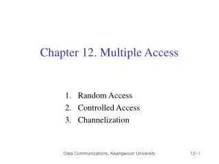
Chapter 12 Multiple Access
Multiple Access • Data Link layer divided into two sublayers. • The upper sublayer is responsible for datalink control, • The lower sublayer is responsible for resolving access to the shared media. Figure 12.1 Data link layer divided into two functionality-oriented sublayers
Taxonomy of multiple-access protocols • Multiple-Access Protocol • When nodes or stations are connected and use a common link, called a multipoint or broadcast link, • We need a multiple-access protocol to coordinate access to the link. Figure 12.2 Taxonomy of multiple-access protocols discussed in this chapter
12-1 RANDOM ACCESS Inrandom accessorcontentionmethods, no station is superior to another station and none is assigned the control over another. No station permits, or does not permit, another station to send. At each instance, a station that has data to send uses a procedure defined by the protocol to make a decision on whether or not to send. Topics discussed in this section: ALOHACarrier Sense Multiple Access Carrier Sense Multiple Access with Collision Detection Carrier Sense Multiple Access with Collision Avoidance
Random Access • Random Access • In a Random access method,each station has the right to the medium without being controlled by any other station. • If more than one station tries to send, there is an access conflict – COLLISION – and the frames will be either destroyed or modified. • To avoid access conflict, each station follows a procedure. • When can the station access the medium ? • What can the station do if the medium is busy ? • How can the station determine the success or failure of the transmission ? • What can the station do if there is an access conflict ?
ALOHA network – Multiple Access • The earliest random-access method, was developed at the Univ. of • Hawaii in the early 1970s. • Base station is central controller • Base station acts as a hop • Potential collisions, all incoming data is @ 407 MHz
ALOHA • Pure ALOHA Random Access • Each station sends a frame whenever it has a frames to send. • However, there is only one channel to share and there is the possibility of collision between frames from different stations. Figure 12.3 Frames in a pure ALOHA network
ALOHA Figure 12.4 Procedure for pure ALOHA protocol
ALOHA Protocol Rule • Acknowledgement • After sending the frame, the station waits for an acknowledgment • If it does not receive an acknowledgement during the 2 times the maximum propagation delay between the two widely separated stations (2 x Tp) • It assumes that the frame is lost; it tries sending again after a random amount of time (TB =R x TP , or R x Tfr ). • Tp (Maximum propagation time)= distance / propagation speed • TB (Back off time) : common formula is binary exponential back-off • R is random number chosen between 0 to 2k - 1 • K is the number of attempted unsuccessful transmissions • Tfr (the average time required to send out a frame)
ALOHA Figure 12.5 Vulnerable time for pure ALOHA protocol
ALOHA The throughput for pure ALOHA isS = G × e −2G . The maximum throughput Smax = 0.184 when G= (1/2). * If one-half a frame is generated during one frame transmission time, then 18.4 percent of these frames reach their destination successfully. • S is the average number of successful transmissions, called throughput. • G is the average number of frames generated by the system during one frame transmission time.
Slotted ALOHA • Slotted ALOHA • We divide the time into slots of Tfr s and force the station to send only at the beginning of the time slot. Figure 12.6 Frames in a slotted ALOHA network
Note Slotted ALOHA The throughput for slotted ALOHA isS = G × e−G . The maximum throughputSmax = 0.368when G = 1. • If a frame is generated during one frame transmission time, • then 36.8 percent of these frames reach their destination successfully.
Slotted ALOHA • Slotted ALOHA vulnerable time = Tfr Figure 12.7 Vulnerable time for slotted ALOHA protocol
Carrier Sense Multiple Access (CSMA) • To minimize the chance of collision and, therefore, increase the performance, the CSMA method was developed. • CSMA is based on the principle “sense before transmit” or “listen before talk.” • CSMA can reduce the possibility of collision, but it cannot eliminate it. • The possibility of collision still exists because of propagation delay; a station may sense the medium and find it idle, only because the first bit sent by another station has not yet been received.
Carrier Sense Multiple Access (CSMA) B C Figure 12.8 Space/time model of the collision in CSMA
Carrier Sense Multiple Access (CSMA) (TP) Figure 12.9 Vulnerable time in CSMA
Persistence methods • Persistence strategy defines the procedures for a station that senses a busy medium. • Three strategies have been developed; • 1-persistent method : after the station finds the line idle, it sends its frame immediately (with probability 1) • non-persistent method : • a station that has a frame to send senses the line. • If the line is idle, it sends immediately. • If the line is not idle, it waits a random amount of time and then senses the line again. • p-persistent method : After the station finds the line idle, • With probability p, the station sends its frames • With probability q=1-p, the station waits for the beginning of the next time slot and checks the line again.
Carrier Sense Multiple Access (CSMA) Figure 12.10 Behavior of three persistence methods
Carrier Sense Multiple Access (CSMA) Figure 12.11 Flow diagram for three persistence methods
CSMA with Collision Detection (CSMA/CD) • CSMA/CD adds a procedure to handle the collision. • A station monitors the medium after it sends a frame to see if the transmission was successful. • If so, the station is finished. • If there is a collision, the frame is sent again. Figure 12.12 Collision of the first bit in CSMA/CD
CSMA with Collision Detection (CSMA/CD) • Minimum Frame Size • For CSMA/CD to work, we need a restriction on the frame size. • The frame transmission time Tfr must be at least two times the maximum propagation time Tp . Figure 12.13 Collision and abortion in CSMA/CD
CSMA with Collision Detection (CSMA/CD) Figure 12.14 Flow diagram for the CSMA/CD
CSMA with Collision Detection (CSMA/CD) Figure 12.15 Energy level during transmission, idleness, or collision
CSMA with Collision Avoidance (CSMA/CA) • CSMA/CA was invented for the wireless networks to avoid collisions. • Collisions are avoided through the use of CSMA/CA’s three strategies: • The interframe space, the contention window, and acknowledgments. Figure 12.16 Timing in CSMA/CA
Note CSMA with Collision Detection (CSMA/CD) In CSMA/CA, the IFS can also be used to define the priority of a station or a frame.
Note CSMA with Collision Detection (CSMA/CD) In CSMA/CA, if the station finds the channel busy, it does not restart the timer of the contention window; it stops the timer and restarts it when the channel becomes idle.
CSMA with Collision Detection (CSMA/CD) Figure 12.17 Flow diagram for CSMA/CA
12-2 CONTROLLED ACCESS Incontrolled access, the stations consult one another to find which station has the right to send. A station cannot send unless it has been authorized by other stations. We discuss three popular controlled-access methods. Topics discussed in this section: ReservationPollingToken Passing
Reservation • A station need to make a reservation before sending data • In each interval, a reservation frame precedes the data frames sent in that interval. • If there are N stations in the system, there are exactly N reservation minislots in the reservation frame. Each minislot belongs to a station. • When a station needs to send a data frame, it makes a reservation in its own minislot. • The stations that have made reservations can send their data frames after the reservation frame. Figure 12.18 Reservation access method
Polling • Polling works with topologies in which one device is designed as a Primary Station and the other devices are Secondary Station. • The primary device controls the link; • The secondary devices follow its instruction. • Poll function : If the primary wants to receive data, it asks the secondaries if they have anything to send. • Select function : If the primary wants to send data, it tells the secondary to get ready to receive.
Polling Figure 12.19 Select and poll functions in polling access method
Token-passing network • A station is authorized to send data when it receives a special frame called a token
Token-passing network Figure 12.20 Logical ring and physical topology in token-passing access method
12-3 CHANNELIZATION Channelizationis a multiple-access method in which the available bandwidth of a link is shared in time, frequency, or through code, between different stations. In this section, we discuss three channelization protocols. Topics discussed in this section: Frequency-Division Multiple Access (FDMA)Time-Division Multiple Access (TDMA) Code-Division Multiple Access (CDMA)
FDMA • The available bandwidth is shared by all stations. • The FDMA is a data link layer protocol that uses FDM at the physical layer In FDMA, the available bandwidth of the common channel is divided into bands that are separated by guard bands.
FDMA Figure 12.21 Frequency-division multiple access (FDMA)
TDMA • The entire bandwidth is just one channel. • Stations share the capacity of the channel in time In TDMA, the bandwidth is just one channel that is timeshared between different stations.
FDMA Figure 12.22 Time-division multiple access (TDMA)
CDMA • CDMA differs from FDMA because only one channel occupies the entire bandwidth of the link. • It differs from TDMA because all stations can send data simultaneously; there is no time sharing. In CDMA, one channel carries all transmissions simultaneously.
CDMA • The assigned codes have two properties. • If we multiply each code by another, we get 0, • 2. If we multiply each code by itself, we get 4 • (the number of stations) • ex) Data = (d1 c1 + d2 c2 + d3 c3 + d4 c4 ) x c1 = 4 x d1 Figure 12.23 Simple idea of communication with code
CDMA • CDMA is based on coding theory • Each station is assigned a code, which is a sequence of numbers called chips. Figure 12.24 Chip sequences
Properties of Orthogonal Sequences • Orthogonal sequences (1) Inner-product of two equal sequences ○ A•A = N ○ If we multiply two different sequences, element by element, and add the results, we get 0. A•B = 0 (2) A•(-A) = -N
CDMA – Data Representation • When a station is idle, it sends no signal, which is represented by a 0. Figure 12.25 Data representation in CDMA
Encoding and Decoding Figure 12.26 Sharing channel in CDMA
Encoding and Decoding Figure 12.27 Digital signal created by four stations in CDMA
CDMA - Encoding Rules • Showing how four stations share the link during 1-bit interval. • CDMA Multiplexer
CDMA - Encoding Rules 2 Figure 12.28 Decoding of the composite signal for one in CDMA
CDMA - Encoding Rules • CDMA Demultiplexer +
CDMA - Sequence Generation • To generate sequences, we use a Walsh table, a two-dimensional table with an equal number of rows and columns. • Each row is a sequence of chips Figure 12.29 General rule and examples of creating Walsh tables