Download
1 / 53
530 likes | 538 Vues
http://www.ugrad.cs.ubc.ca/~cs314/Vjan2005. Virtual Trackball, Scientific Visualization Week 12, Wed Mar 30. News. reminder: my office hours today 3:45 proposals: email out to several of you midterm 2 solutions out. Review: Splines. spline is parametric curve defined by control points

E N D
http://www.ugrad.cs.ubc.ca/~cs314/Vjan2005 Virtual Trackball, Scientific VisualizationWeek 12, Wed Mar 30
News • reminder: my office hours today 3:45 • proposals: email out to several of you • midterm 2 solutions out
Review: Splines • spline is parametric curve defined by control points • knots: control points that lie on curve • engineering drawing: spline was flexible wood, control points were physical weights A Duck (weight) Ducks trace out curve
Review: Hermite Spline • user provides • endpoints • derivatives at endpoints
Review: Bézier Curves • four control points, two of which are knots • more intuitive definition than derivatives • curve will always remain within convex hull (bounding region) defined by control points
Review: Basis Functions • point on curve obtained by multiplying each control point by some basis function and summing
Review: Comparing Hermite and Bézier Bézier Hermite
M12 P1 P2 M012 M0123 M123 M01 M23 P0 P3 Review: Sub-Dividing Bézier Curves • find the midpoint of the line joining M012, M123. call it M0123
Review: de Casteljau’s Algorithm • can find the point on Bézier curve for any parameter value t with similar algorithm • for t=0.25, instead of taking midpoints take points 0.25 of the way M12 P2 P1 M23 t=0.25 M01 P0 P3 demo: www.saltire.com/applets/advanced_geometry/spline/spline.htm
continuity definitions C0: share join point C1: share continuous derivatives C2: share continuous second derivatives Review: Continuity • piecewise Bézier: no continuity guarantees
Review: B-Spline • C0, C1, and C2 continuous • piecewise: locality of control point influence
Virtual Trackball • interface for spinning objects around • drag mouse to control rotation of view volume • rolling glass trackball • center at screen origin, surrounds world • hemisphere “sticks up” in z, out of screen • rotate ball = spin world
Virtual Trackball • know screen click: (x, 0, z) • want to infer point on trackball: (x,y,z) • ball is unit sphere, so ||x, y, z|| = 1.0 • solve for y eye image plane
Trackball Rotation • correspondence: • moving point on plane from (x, 0, z) to (a, 0, c) • moving point on ball from p1 =(x, y, z) to p2 =(a, b, c) • correspondence: • translating mouse from p1 (mouse down) to p2 (mouse up) • rotating about the axis n = p1 x p2
Trackball Computation • user defines two points • place where first clicked p1 = (x, y, z) • place where released p2 = (a, b, c) • create plane from vectors between points, origin • axis of rotation is plane normal: cross product • (p1 - - o) x (p2 - - o): p1 x p2 if origin = (0,0,0) • amount of rotation depends on angle between lines • p1 • p2 = |p1| |p2| cos θ • |p1 x p2 | = |p1| |p2| sin θ • compute rotation matrix, use to rotate world
Reading • FCG Chapter 23
Surface Graphics • objects explicitly defined by surface or boundary representation • mesh of polygons 1000 polys 200 polys 15000 polys
Surface Graphics • pros • fast rendering algorithms available • hardware acceleration cheap • OpenGL API for programming • use texture mapping for added realism • cons • discards interior of object, maintaining only the shell • operations such cutting, slicing & dissection not possible • no artificial viewing modes such as semi-transparencies, X-ray • surface-less phenomena such as clouds, fog & gas are hard to model and represent
Volume Graphics • for some data, difficult to create polygonal mesh • voxels: discrete representation of 3D object • volume rendering: create 2D image from 3D object • translate raw densities into colors and transparencies • different aspects of the dataset can be emphasized via changes in transfer functions
Volume Graphics • pros • formidable technique for data exploration • cons • rendering algorithm has high complexity! • special purpose hardware costly (~$3K-$10K) volumetric human head (CT scan)
Isosurfaces • 2D scalar fields: isolines • contour plots, level sets • topographic maps • 3D scalar fields: isosurfaces
Volume Graphics: Examples industrial CT - structural failure, security applications anatomical atlas from visible human (CT & MRI) datasets shockwave visualization: simulation with Navier-Stokes PDEs flow around airplane wing
Isosurface Extraction • array of discrete point samples at grid points • 3D array: voxels • find contours • closed, continuous • determined by iso-value • several methods • marching cubes is most common 0 1 1 3 2 1 3 6 6 3 3 7 9 7 3 2 7 8 6 2 1 2 3 4 3 Iso-value = 5
MC 1: Create a Cube • consider a cube defined by eight data values (i,j+1,k+1) (i+1,j+1,k+1) (i,j,k+1) (i+1,j,k+1) (i,j+1,k) (i+1,j+1,k) (i,j,k) (i+1,j,k)
MC 2: Classify Each Voxel • classify each voxel according to whether lies • outside the surface (value > iso-surface value) • inside the surface (value <= iso-surface value) 10 10 Iso=9 5 5 10 8 Iso=7 8 8 =inside =outside
MC 3: Build An Index • binary labeling of each voxel to create index v8 v7 11110100 inside =1 v4 outside=0 v3 v5 v6 00110000 v1 v2 Index: v3 v5 v6 v1 v2 v4 v7 v8
MC 4: Lookup Edge List • use index to access array storing list of edges • all 256 cases can be derived from 15 base cases
MC 4: Example • index = 00000001 • triangle 1 = a, b, c c a b
MC 5: Interpolate Triangle Vertex • for each triangle edge • find vertex location along edge using linear interpolation of voxel values i+1 i x =10 =0 T=8 T=5
MC 6: Compute Normals • calculate the normal at each cube vertex • use linear interpolation to compute the polygon vertex normal
Direct Volume Rendering • do not compute surface
Rendering Pipeline Classify
Classification • data set has application-specific values • temperature, velocity, proton density, etc. • assign these to color/opacity values to make sense of data • achieved through transfer functions
Transfer Functions • map data value to color and opacity
a(f) RGB(f) shading, compositing… Human Tooth CT Transfer Functions RGB a f Gordon Kindlmann
Setting Transfer Functions • can be difficult, unintuitive, and slow a a f f a a f f Gordon Kindlmann
Rendering Pipeline Classify Shade
Light Effects • usually only consider reflected part Light reflected specular Light absorbed ambient diffuse transmitted Light=refl.+absorbed+trans. Light=ambient+diffuse+specular
Rendering Pipeline Classify Shade Interpolate
given: 1D • given: • needed: • needed: Interpolation 2D linear nearest neighbor
Rendering Pipeline Classify Shade Interpolate Composite
Volume Rendering Algorithms • ray casting • image order, forward viewing • splatting • object order, backward viewing • texture mapping • object order • back-to-front compositing
Ray Traversal Schemes Intensity Max Average Accumulate First Depth
Ray Traversal - First • first: extracts iso-surfaces (again!) Intensity First Depth
Ray Traversal - Average • average: looks like X-ray Intensity Average Depth
Ray Traversal - MIP • max: Maximum Intensity Projection • used for Magnetic Resonance Angiogram Intensity Max Depth