Download
1 / 58
590 likes | 742 Vues
Melanie Tory Acknowledgments: Torsten M öller (Simon Fraser University) Raghu Machiraju (Ohio State University) Klaus Mueller (SUNY Stony Brook). Scientific Visualization. Overview. What is SciVis? Data & Applications Iso-surfaces Direct Volume Rendering Vector Visualization Challenges.

E N D
Melanie Tory Acknowledgments: Torsten Möller (Simon Fraser University) Raghu Machiraju (Ohio State University)Klaus Mueller (SUNY Stony Brook) Scientific Visualization
Overview • What is SciVis? • Data & Applications • Iso-surfaces • Direct Volume Rendering • Vector Visualization • Challenges
SciVis InfoVis Difference between SciVis and InfoVis Parallel Coordinates Direct Volume Rendering [Hauser et al.,Vis 2000] [Fua et al., Vis 1999] Isosurfaces Glyphs Scatter Plots Line Integral Convolution [http://www.axon.com/gn_Acuity.html] Node-link Diagrams [Cabral & Leedom,SIGGRAPH 1993] Streamlines [Lamping et al., CHI 1995] [Verma et al.,Vis 2000]
Difference between SciVis and InfoVis • Card, Mackinlay, & Shneiderman: • SciVis: Scientific, physically based • InfoVis: Abstract • Munzner: • SciVis: Spatial layout given • InfoVis: Spatial layout chosen • Tory & Möller: • SciVis: Spatial layout given + Continuous • InfoVis: Spatial layout chosen + Discrete • Everything else -- ?
Overview • What is SciVis? • Data & Applications • Iso-surfaces • Direct Volume Rendering • Vector Visualization • Challenges
Medical Scanning • MRI, CT, SPECT, PET, ultrasound
Medical Scanning - Applications • Medical education for anatomy, surgery, etc. • Illustration of medical procedures to the patient
Medical Scanning - Applications • Surgical simulation for treatment planning • Tele-medicine • Inter-operative visualization in brain surgery, biopsies, etc.
Biological Scanning • Scanners: Biological scanners, electronic microscopes, confocal microscopes • Apps – physiology, paleontology, microscopic analysis…
Industrial Scanning • Planning (e.g., log scanning) • Quality control • Security (e.g. airport scanners)
Scientific Computation - Domain • Mathematical analysis • ODE/PDE (ordinary and partialdifferential equations) • Finite element analysis (FE) • Supercomputer simulations
Scientific Computation - Apps • Flow Visualization
Overview • What is SciVis? • Data & Applications • Iso-surfaces • Direct Volume Rendering • Vector Visualization • Challenges
Isosurfaces - Examples Isolines Isosurfaces
Isosurface Extraction 0 1 1 3 2 • by contouring • closed contours • continuous • determined by iso-value • several methods • marching cubes is most common 1 3 6 6 3 3 7 9 7 3 2 7 8 6 2 1 2 3 4 3 Iso-value = 5
MC 1: Create a Cube • Consider a Cube defined by eight data values: (i,j+1,k+1) (i+1,j+1,k+1) (i,j,k+1) (i+1,j,k+1) (i,j+1,k) (i+1,j+1,k) (i,j,k) (i+1,j,k)
MC 2: Classify Each Voxel • Classify each voxel according to whether it liesoutside the surface (value > iso-surface value)inside the surface (value <= iso-surface value) 10 10 Iso=9 5 5 10 8 Iso=7 8 8 =inside =outside
MC 3: Build An Index • Use the binary labeling of each voxel to create an index v8 v7 11110100 inside =1 v4 outside=0 v3 v5 v6 00110000 v1 v2 Index: v3 v5 v6 v1 v2 v4 v7 v8
MC 4: Lookup Edge List • For a given index, access an array storing a list of edges • all 256 cases can be derived from 15 base cases
MC 4: Example • Index = 00000001 • triangle 1 = a, b, c c a b
MC 5: Interp. Triangle Vertex • For each triangle edge, find the vertex location along the edge using linear interpolation of the voxel values i+1 i x =10 =0 T=8 T=5
MC 6: Compute Normals • Calculate the normal at each cube vertex • Use linear interpolation to compute the polygon vertex normal
Overview • What is SciVis? • Data & Applications • Iso-surfaces • Direct Volume Rendering • Vector Visualization • Challenges
Rendering Pipeline (RP) Classify
Classification • original data set has application specific values (temperature, velocity, proton density, etc.) • assign these to color/opacity values to make sense of data • achieved through transfer functions
a(f) RGB(f) Shading, Compositing… Human Tooth CT Transfer Functions (TF’s) RGB a • Simple (usual) case: Map data value f to color and opacity f Gordon Kindlmann
TF’s • Setting transfer functions is difficult, unintuitive, and slow a a f f a a f f Gordon Kindlmann
Transfer Function Challenges • Better interfaces: • Make space of TFs less confusing • Remove excess “flexibility” • Provide guidance • Automatic / semi-automatic transfer function generation • Typically highlight boundaries Gordon Kindlmann
Rendering Pipeline (RP) Classify Shade
Light Effects • Usually only considering reflected part Light reflected specular Light absorbed ambient diffuse transmitted Light=refl.+absorbed+trans. Light=ambient+diffuse+specular
Rendering Pipeline (RP) Classify Shade Interpolate
1D • Given: • Needed: • Needed: Interpolation 2D • Given:
Interpolation • Very important; regardless of algorithm • Expensive => done very often for one image • Requirements for good reconstruction • performance • stability of the numerical algorithm • accuracy Linear Nearest neighbor
Rendering Pipeline (RP) Classify Shade Interpolate Composite
Ray Traversal Schemes Intensity Max Average Accumulate First Depth
Ray Traversal - First Intensity • First: extracts iso-surfaces (again!)done by Tuy&Tuy ’84 First Depth
Ray Traversal - Average Intensity • Average: produces basically an X-ray picture Average Depth
Ray Traversal - MIP Intensity • Max: Maximum Intensity Projectionused for Magnetic Resonance Angiogram Max Depth
Ray Traversal - Accumulate Intensity • Accumulate: make transparent layers visible!Levoy ‘88 Accumulate Depth
1.0 Volumetric Ray Integration color opacity object (color, opacity)
Overview • What is SciVis? • Data & Applications • Iso-surfaces • Direct Volume Rendering • Vector Visualization • Challenges
Flow Visualization • Traditionally – Experimental Flow Vis • Now – Computational Simulation • Typical Applications: • Study physics of fluid flow • Design aerodynamic objects
Glyphs (arrows) Techniques Contours Jean M. Favre Streamlines
Techniques - Stream-ribbon • Trace one streamline and a constant size vector with it • Allows you to see places where flow twists
Techniques - Stream-tube • Generate a stream-line and widen it to a tube • Width can encode another variable
Mappings - Flow Volumes • Instead of tracing a line - trace a small polyhedron