Download
1 / 55
570 likes | 597 Vues
Raster Analysis. Ming-Chun Lee. Raster Analysis. Performed on cells and grids. Raster cells store data Nominal – land use Ordinal – street classification Interval/Ratio – temperature, elevation

E N D
Raster Analysis Ming-Chun Lee
Raster Analysis • Performed on cells and grids. • Raster cells store data • Nominal – land use • Ordinal – street classification • Interval/Ratio – temperature, elevation • Perform analysis based on manipulations on cell values for a single raster layer or multiple layers.
Why use Raster GIS • Raster is better suited for spatially continuous data • Elevations, pH, air pressure, temperature, salinity • Raster is better for creating visualizations and modeling environmental phenomena • Raster data is a simplified realization of the world, and allows for fast and efficient processing
Map Algebra • Cell by Cell combination of raster data layers using mathematical operations • one layer • multiple layers • Each number represents a value at a raster cell location • Simple operations can be applied to each number • Raster layers may be combined through operations • Addition, subtraction and multiplication
5 7 4 Map Algebra 4 1 3 2 3 6 Input 1 4 2 2 6 1 2 3 + 6 3 3 4 2 1 6 2 Input 2 4 6 4 3 1 3 2 4 = 7 7 6 6 13 5 7 7 Output 6 10 8 5 2 10 5 5
Map Algebra • The computer will allow you to perform virtually any mathematical calculation • beware: some will make sense, others won’t. • For example, water = 0, land = 1. Then, you can multiply this grid with an elevation map. The output will include 0’s where water existed (x * 0 = 0), and the original elevation value where land existed (x * 1 = x) • Or, you can add the elevations and the grid with 0’s and 1’s together (but, it would be meaningless!)
Map Algebra Grid1 * Grid2 = Grid3 Grid1 Grid2 1 0 * = 0 Grid3
Map Algebra • Multiple grid themes share the same X, Y coordinate space • A single output grid theme is the result of the multiple grids
Map Algebra • Mathematical Operators: • Arithmetic +, -, *, / • Boolean AND, OR, NOT, XOR • Relational =, <, >, ≤, ≥, <> • Algebraic Functions Powers & Roots, Trigonometry, Logarithm
Scope of Computations • Local Functions • Process cells on a cell-by-cell basis. • only use data in a single cell to calculate an output value • Focal/Neighborhood Functions • Process data for each pixel using the attribute values of the neighboring cells of that pixel. • Zonal Functions • Process cells on the basis of zones. • Global Functions • Process data at each pixel on the output grid using entire source grid.
5 7 4 Local Functions input 25 49 output = sqr(input) 16
Local Functions • Operations that modify a cell on a single grid • Data type changes • Arithmetic operations • Converting one value to another according to a rule (Recode) • Local operations on multiple layers • Map algebra (Output = f(Input1, Input2,…) • Functions may be mathematical or logical
Local Functions Single grid Multiple grid (addition)
5 7 4 Focal/Neighborhood Functions input 11 16 output = focalsum(input)
Focal/Neighborhood Functions • Moving window • Assigns the value of a neighborhood of grid cells to one particular grid cell (kernel) • Useful for calculating local statistical functions
5 7 4 Zonal Functions input Zone 2 zone Zone 1 output = zonalsum(zone, input) 9 7 7 7 9 7 7 7 9 9 9 7 9 9 9 7
Zonal Functions • Output value at each location depends on the values of all the input cells in an input value grid that shares the same input value zone • Type of complex neighborhood function • use complex neighborhoods or zones
input Input_zone 535.54 127 6280 766.62 160 10800
5 7 4 Global Functions input 6 7 8 9 5 6 7 8 output = trend(input) 4 5 6 7 4 5 6 6
Global Functions • Output value of each location is potentially a function of all the cells in the input grid • e.g. distance functions, surfaces, interpolation, etc.
Distance to Features • Cell value is the Distance from the Cell Center to the Nearest Feature(s) in a Specified Layer • Physical distance– equivalent to buffers • Cost distance • Requires a cost grid as input • Cost grid contains costs for unit distance • Cost distance between two cells is the average of the two values multiplied by the distance between them • Total cost is calculated to source cells.
Interpolation Between Features • Interpolation predicts values for cells in a raster from a limited number of sample data points. • Elevation, rainfall, chemical concentration, noise level • Average of Nearby Features’ Values, Weighted by Distance, Regardless of Density • Example: Number of Bus Routes Serving a Neighborhood!
Density of Features • Value Assigned Based on the Neighborhood Density of a Feature • Can be Weighted on an Attribute Value • Example: Estimate a Population Density Surface Using Census Tract Population • Another Example – Bus Service Density
Spatial Analyst functions • Find Distance • Calculate Density • Interpolate Surface • Derive Slope, Aspect • Create Contour • Cell Statistics • Summarize Zones • Tabulate Areas • Map Query, Calculator • Neighborhood Statistics • Reclassify
Raster-based Analysis • Finding potential sites for a new school • (ESRI: Using ArcGIS Spatial Analyst) • Criteria: • On flat land • Near recreation sites • Away from existing schools • Land use in terms of cost • Agricultural – cheapest • Barren land • Brush/Transitional • Forest • Built up – most expensive
Weighting and Combining Datasets • Weights: • Dist to Rec_sites: 0.5 • Dist to schools: 0.25 • Landuse: 0.125 • Slope: 0.125
Cost Layer • Slope: • High values (10) to steeper slopes • Land Use: • Agricultural: 4 • Brush/Transitional: 5 • Barren land: 6 • Forest: 8 • Built up: 9 • Water: 10