Advanced Raster Analysis with Map Algebra in Python
460 likes | 553 Vues
Learn complex raster modeling with Map Algebra, managing rasters, and optimization techniques in Python for efficient spatial analysis. Access advanced spatial tools and execute complex expressions easily.

Advanced Raster Analysis with Map Algebra in Python
E N D
Presentation Transcript
July 2012 Python - Raster Analysis Kevin M. Johnston Ryan DeBruyn
The problem that is being addressed • You have a complex modeling problem • You are mainly working with rasters • Some of the spatial manipulations that you trying to implement are difficult or not possible using standard ArcGIS tools • Due to the complexity of the modeling problem, processing speed is a concern
Outline • Managing rasters with management tools and performing analysis with Map Algebra • How to access the analysis capability – Demonstration • Complex expressions and optimization – Demonstration • Additional modeling capability: classes – Demonstration • Full modeling control: NumPy arrays – Demonstration • Pre-10 Map Algebra
The complex model Emerald Ash Borer Originated in Michigan Infest ash trees 100% kill Coming to Vermont
The ash borer model • Movement by flight • 20 km per year • Vegetation type and ash density (suitability surface) • Movement by hitchhiking • Roads • Camp sites • Mills • Population • Current location of the borer (suitability surface) • Random movement
Raster analysis • To prepare and manage raster data • Displaying • Adding, copying, deleting, etc. • Mosaic, Clip, etc. • Raster object • NumPy, ApplyEnvironment, etc. • To perform the analysis use raster analysis/modeling • Spatial Analyst • Map Algebra
What is Map Algebra • Simple and powerful algebra to execute Spatial Analyst tools, operators, and functions to perform geographic analysis • The strength is in creating complex expressions • Available through Spatial Analyst module • Integrated in Python (all modules available)
Importing Spatial Analyst • Module of ArcPy site package • Like all modules must be imported • To access the operators and tools in an algebraic format the imports are important import arcpy from arcpy import env # Analysis environment from arcpy.sa import *
General syntax • Map Algebra available through an algebraic format • Simplest form: output raster is specified to the left of an equal sign and the tool and its parameters on the right • Comprised of: • Input data • Operators • Tools • Parameters • Output from arcpy.sa import * outRas = Slope(“indem”)
Input data • Input elements • Rasters • Features • Numbers • Constants • Objects • Variables outRas = Slope(“inraster”) Tip: Names are quoted – if in workspace no path is necessary (or if using Python window and the layer is in the TOC)
Map Algebra operators • Symbols for mathematical operations • Many operators in both Python and Spatial Analyst • Cast the raster (Raster class constructor) indicates operator should be applied to rasters outRas = Raster(“inraster1”) + Raster(“inraster2”) outRas2 = Raster(“inraster”) + 8
Map Algebra tools • All the tools that output a raster are available (e.g., Sin, Slope, Reclassify, etc.) • Can use any Geoprocessing tools outRas = Aspect(“inraster”) Tip: Tool names are case sensitive
Tool parameters • Defines how the tool is to be executed • Each tool has its own unique set of parameters • Some are required, others are optional • Numbers, strings, and objects (classes) outRas = Slope(“inraster”, “PERCENT_RISE”) Tip: Keywords are in quotes and it is recommended they are capitalized
Map Algebra output • Stores the results as a Raster object • Object with methods and properties • Generally, in Python window and scripting the output is temporary outRas = Hillshade(“inraster”)
Access to Map Algebra • Raster Calculator • Spatial Analyst tool • Easy to use calculator interface • Stand alone or in ModelBuilder • Python window • Single expression or simple exploratory models • Scripting • Complex models • Line completion and colors
Demo 1: Data management Raster management tools Raster Calculator Python window ModelBuilder Simple expressions
Outline • Managing rasters with management tools and performing analysis with Map Algebra • How to access the analysis capability - Demonstration • Complex expressions and optimization - Demonstration • Additional modeling capability: classes - Demonstration • Full modeling control: NumPy arrays - Demonstration • Pre-10 Map Algebra
Complex expressions • Multiple operators and tools can be implemented in a single expression • Output from one expression can be the input to a subsequent expression Tip: It is a good practice to set the input to a variable and use the variable in the expression
More on the raster object • A variable with a pointer to a dataset • Output from a Map Algebra expression or from an existing dataset • The associated dataset is temporary (when created from Map Algebra) but has a save method • A series of properties describing the associated dataset • Description of raster (e.g., number of rows) • Description of the values (e.g., mean)
Optimization • A series of local tools (Abs, Sin, Cell Statistics, etc.) and operators can be optimized • Work on a per-cell basis • When entered into a single expression each tool and operator is processed on a per cell basis
The iterative aspects of the ash borer model • Movement by flight • Depends on the year how far it can move in a time step • “Is there a borer in my neighborhood” • “Will I accept it” – suitability surface • Movement by hitchhiking • Based on highly susceptible areas • Nonlinear decay • Random points and check susceptibility • Random movement • Nonlinear decay from known locations (NumPy array)
Demo 2: Movement by hitchhiking Roads, Campsites, Mills, Population,and current location (suitability) Complex expressions Raster object Optimization
Outline • Managing rasters with management tools and performing analysis with Map Algebra • How to access the analysis capability - Demonstration • Complex expressions and optimization - Demonstration • Additional modeling capability: classes - Demonstration • Full modeling control: NumPy arrays - Demonstration • Pre-10 Map Algebra
Classes • Objects that are used as parameters to tools • Varying number of arguments depending on the selected parameter choice (neighborhood type) • The number of entries into the parameters can vary depending on the specific situation (a remap table) • More flexible • Query the individual arguments
Classes - Categories • General • Fuzzy classes - Time classes • Hf classes - VF classes • KrigingModel classes - Radius classes • Nbr classes • Composed of lists • Topo classes • Composed of lists within lists • Reclass - Weighted reclass tables • Topo classes (a subset)
Classes - Categories • Creating • Querying • Changing arguments neigh = NbrCircle(4, “MAP”) radius = neigh.radius neigh.radius = 6
Vector integration • Feature data is required for some Spatial Analyst Map Algebra • IDW, Kriging, etc. • Geoprocessing tools that operate on feature data can be used in an expression • Buffer, Select, etc.
The iterative aspects of the ash borer model • Movement by flight • Depends on the year how far it can move in a time step • “Is there a borer in my neighborhood” • “Will I accept it” – suitability surface • Movement by hitchhiking • Based on highly susceptible areas • Nonlinear decay • Random points and check susceptibility • Random movement • Nonlinear decay from known locations (NumPy array)
Demo 3: Movement by flight 20 km per year Vegetation type/ash density (suitability) Classes Using variables Vector integration
Outline • Managing rasters with management tools and performing analysis with Map Algebra • How to access the analysis capability - Demonstration • Complex expressions and optimization - Demonstration • Additional modeling capability: classes - Demonstration • Full modeling control: NumPy arrays - Demonstration • Pre-10 Map Algebra
NumPy Arrays • A generic Python storage mechanism • Create custom tool • Access the wealth of free tools built by the scientific community • Clustering • Filtering • Linear algebra • Optimization • Fourier transformation • Morphology
NumPy Arrays • Two tools • RasterToNumPyArray • NumPyArrayToRaster Raster Numpy Array 1 3 3 1 3 3 2 4 4 2 4 4
The iterative aspects of the ash borer model • Movement by flight • Depends on the year how far it can move in a time step • “Is there a borer in my neighborhood” • “Will I accept it” – suitability surface • Movement by hitchhiking • Based on highly susceptible areas • Nonlinear decay • Random points and check susceptibility • Random movement • Nonlinear decay from known locations (NumPy array)
Demo 4: The random movement Random movement based on nonlinear decay from existing locations Custom function NumPy array
Outline • Managing rasters with management tools and performing analysis with Map Algebra • How to access the analysis capability - Demonstration • Complex expressions and optimization - Demonstration • Additional modeling capability: classes - Demonstration • Full modeling control: NumPy arrays - Demonstration • Pre-10 Map Algebra
Pre-10.0 Map Algebra • Similar to Map Algebra 10.0 • Faster, more powerful, and easy to use (line completion, colors) • Any changes are to take advantage of the Python integration • Raster Calculator at 10.0 replaces the Raster Calculator from the tool bar, SOMA, and MOMA • SOMA in existing models will still work
Summary • When the problem become more complex you may need additional capability provided by Map Algebra • Map Algebra powerful, flexible, easy to use, and integrated into Python • Accessed through: Raster Calculator, Python window, ModelBuilder (through Raster Calculator), and scripting • Raster object and classes • Create models that can better capture interaction of phenomena
ArcGIS Spatial Analyst Technical Sessions • An Introduction - Rm 15B Tuesday, July 24, 8:30AM – 9:45AM Wed, July 25, 1:30PM – 2:45PM • Suitability Modeling - Rm 15A Tuesday, July 24, 10:15AM – 11:30AM Thursday, July 26, 3:15PM – 4:30PM • Raster Analysis with Python – Ball06 E Tuesday, July 23, 3:15PM – 4:30PM Thursday, July 25, 3:15PM – 4:30PM • Creating Surfaces – Rm 15A Wednesday, July 25, 8:30PM – 9:45PM
ArcGIS Spatial Analyst Short Technical Sessions • Creating Watersheds and Stream Networks – Rm 01B Tuesday, July 24, 1:30 PM – 1:50PM • Performing Regression Analysis Using Raster Data – 01A Tuesday, July 24, 9:20AM – 9:40AM
Demo Theater Presentations – Exhibit Hall C • Modeling Rooftop Solar Energy Potential Tuesday, July 24, 11:30AM – 12:00PM • Surface Interpolation in ArcGIS Wednesday, July 25, 1:00PM – 2:00PM • Getting Started with Map Algebra Thursday, July 26, 10:00AM – 11:00AM • Agent-Based Modeling Wednesday, July 25, 12:00PM – 1:00PM
Thank You!...Open to QuestionsPlease fill the evaluations.www.esri.com/ucsessionsurveysFirst Offering ID: XXXX Second Offering ID: XXXX My UC Homepage > “Evaluate Sessions”