Download
1 / 56
640 likes | 968 Vues
Chapter 18 Forecasting. Quantitative Approaches to Forecasting. Components of a Time Series. Measures of Forecast Accuracy. Smoothing Methods. Trend Projection. Trend and Seasonal Components. Regression Analysis. Qualitative Approaches. Forecasting Methods. Forecasting Methods.

E N D
Chapter 18Forecasting • Quantitative Approaches to Forecasting • Components of a Time Series • Measures of Forecast Accuracy • Smoothing Methods • Trend Projection • Trend and Seasonal Components • Regression Analysis • Qualitative Approaches
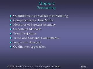
Forecasting Methods Forecasting Methods Quantitative Qualitative Causal Time Series Smoothing Trend Projection Trend Projection Adjusted for Seasonal Influence
Quantitative Approaches to Forecasting • Quantitative methods are based on an analysis of historical data concerning one or more time series. • A time series is a set of observations measured at successive points in time or over successive periods of time. • If the historical data used are restricted to past values of the series that we are trying to forecast, the procedure is called a time series method. • If the historical data used involve other time series that are believed to be related to the time series that we are trying to forecast, the procedure is called a causal method.
Time Series Methods • Three time series methods are: • smoothing • trend projection • trend projection adjusted for seasonal influence
Irregular Trend Cyclical Seasonal Components of a Time Series • The pattern or behavior of the data in a time series has several components. • The four components we will study are:
Components of a Time Series • Trend Component • The trend component accounts for the gradual shifting of the time series to relatively higher or lower values over a long period of time. • Trend is usually the result of long-term factors such as changes in the population, demographics, technology, or consumer preferences.
Components of a Time Series • Cyclical Component • Any regular pattern of sequences of values above and below the trend line lasting more than one year can be attributed to the cyclical component. • Usually, this component is due to multiyear cyclical movements in the economy.
Components of a Time Series • Seasonal Component • The seasonal component accounts for regular patterns of variability within certain time periods, such as a year. • The variability does not always correspond with the seasons of the year (i.e. winter, spring, summer, fall). • There can be, for example, within-week or within-day “seasonal” behavior.
Components of a Time Series • Irregular Component • The irregular component is caused by short-term, unanticipated and non-recurring factors that affect the values of the time series. • This component is the residual, or “catch-all,” factor that accounts for unexpected data values. • It is unpredictable.
Measures of Forecast Accuracy • Mean Squared Error The average of the squared forecast errors for the historical data is calculated. The forecasting method or parameter(s) that minimize this mean squared error is then selected. • Mean Absolute Deviation The mean of the absolute values of all forecast errors is calculated, and the forecasting method or parameter(s) that minimize this measure is selected. (The mean absolute deviation measure is less sensitive to large forecast errors than the mean squared error measure.)
Moving Averages Weighted Moving Averages Exponential Smoothing Smoothing Methods • In cases in which the time series is fairly stable and has no significant trend, seasonal, or cyclical effects, one can use smoothing methods to average out the irregular component of the time series. • Three common smoothing methods are:
Smoothing Methods • Moving Averages The moving averages method consists of computing an average of the most recent n data values for the series and using this average for forecasting the value of the time series for the next period.
Smoothing Methods: Moving Averages • Example: Rosco Drugs Sales of Comfort brand headache medicine for the past ten weeks at Rosco Drugs are shown on the next slide. If Rosco Drugs uses a 3-period moving average to forecast sales, what is the forecast for Week 11?
Smoothing Methods: Moving Averages • Example: Rosco Drugs Week Sales Week Sales 1 2 3 4 5 110 115 125 120 125 6 7 8 9 10 120 130 115 110 130
Smoothing Methods: Moving Averages Week Sales 3MA Forecast 1 2 3 4 5 6 7 8 9 10 11 110 115 125 120 125 120 130 115 110 130 (110 + 115 + 125)/3 116.7 116.7 120.0 123.3 121.7 125.0 121.7 118.3 118.3 120.0 123.3 121.7 125.0 121.7 118.3 118.3
Smoothing Methods • Weighted Moving Averages • To use this method we must first select the number of data values to be included in the average. • Next, we must choose the weight for each of the data values. • The more recent observations are typically given more weight than older observations. • For convenience, the weights usually sum to 1.
Smoothing Methods • Weighted Moving Averages • An example of a 3-period weighted moving average (3WMA) is: 3WMA = .2(110) + .3(115) + .5(125) = 119 Most recent of the three observations Weights (.2, .3, and .5) sum to 1
Smoothing Methods • Exponential Smoothing • This method is a special case of a weighted moving averages method; we select only the weight for the most recent observation. • The weights for the other data values are computed automatically and become smaller as the observations grow older. • The exponential smoothing forecast is a weighted average of all the observations in the time series.
Smoothing Methods To start the calculations, we let F1 = Y1 • Exponential Smoothing Model Ft+1 = aYt + (1 – a)Ft where Ft+1 = forecast of the time series for period t + 1 Yt = actual value of the time series in period t Ft = forecast of the time series for period t a = smoothing constant (0 <a< 1)
Smoothing Methods • Exponential Smoothing Model • With some algebraic manipulation, we can rewrite Ft+1 = aYt + (1 – a)Ft as: Ft+1 = Ft + a(Yt – Ft) • We see that the new forecast Ft+1 is equal to the previous forecast Ft plus an adjustment, which is a times the most recent forecast error, Yt – Ft.
Smoothing Methods: Exponential Smoothing • Example: Rosco Drugs Sales of Comfort brand headache medicine for the past ten weeks at Rosco Drugs are shown on the next slide. If Rosco Drugs uses exponential smoothing to forecast sales, which value for the smoothing constant , .1 or .8, gives better forecasts?
Smoothing Methods: Exponential Smoothing • Example: Rosco Drugs Week Sales Week Sales 1 2 3 4 5 110 115 125 120 125 6 7 8 9 10 120 130 115 110 130
Smoothing Methods: Exponential Smoothing • Exponential Smoothing ( = .1, 1 - = .9) F1 = 110 F2 = .1Y1 + .9F1 = .1(110) + .9(110) = 110 F3 = .1Y2 + .9F2 = .1(115) + .9(110) = 110.5 F4 = .1Y3 + .9F3 = .1(125) + .9(110.5) = 111.95 F5 = .1Y4 + .9F4 = .1(120) + .9(111.95) = 112.76 F6 = .1Y5 + .9F5 = .1(125) + .9(112.76) = 113.98 F7 = .1Y6 + .9F6 = .1(120) + .9(113.98) = 114.58 F8 = .1Y7 + .9F7 = .1(130) + .9(114.58) = 116.12 F9 = .1Y8 + .9F8 = .1(115) + .9(116.12) = 116.01 F10= .1Y9 + .9F9 = .1(110) + .9(116.01) = 115.41
Smoothing Methods: Exponential Smoothing • Exponential Smoothing ( = .8, 1 - = .2) F1 = 110 F2 = .8(110) + .2(110) = 110 F3 = .8(115) + .2(110) = 114 F4 = .8(125) + .2(114) = 122.80 F5 = .8(120) + .2(122.80) = 120.56 F6 = .8(125) + .2(120.56) = 124.11 F7 = .8(120) + .2(124.11) = 120.82 F8 = .8(130) + .2(120.82) = 128.16 F9 = .8(115) + .2(128.16) = 117.63 F10= .8(110) + .2(117.63) = 111.53
Smoothing Methods: Exponential Smoothing • Mean Squared Error In order to determine which smoothing constant gives the better performance, we calculate, for each, the mean squared error for the nine weeks of forecasts, weeks 2 through 10. [(Y2-F2)2 + (Y3-F3)2 + (Y4-F4)2 + . . . + (Y10-F10)2]/9
Smoothing Methods: Exponential Smoothing = .1 = .8 Week (Yt - Ft)2 (Yt - Ft)2 Ft Ft Yt 2 3 4 5 6 7 8 9 10 115 125 120 125 120 130 115 110 130 110.00 110.50 111.95 112.76 113.98 114.58 116.12 116.01 115.41 25.00 210.25 64.80 149.94 36.25 237.73 1.26 36.12 212.87 110.00 114.00 122.80 120.56 124.11 120.82 128.16 117.63 111.53 25.00 121.00 7.84 19.71 16.91 84.23 173.30 58.26 341.27 Sum 974.22 Sum 847.52 MSE Sum/9 108.25 Sum/9 94.17
Trend Projection • If a time series exhibits a linear trend, the method of least squares may be used to determine a trend line (projection) for future forecasts. • Least squares, also used in regression analysis, determines the unique trend line forecast which minimizes the mean square error between the trend line forecasts and the actual observed values for the time series. • The independent variable is the time period and the dependent variable is the actual observed value in the time series.
Trend Projection • Using the method of least squares, the formula for the trend projection is: Tt= b0 + b1t where: Tt = trend forecast for time period t b1 = slope of the trend line b0 = trend line projection for time 0
= average time period for the n observations = average of the observed values for Yt Trend Projection • For the trend projection equation Tt= b0 + b1t where: Yt = observed value of the time series at time period t
Trend Projection • Example: Auger’s Plumbing Service The number of plumbing repair jobs performed by Auger's Plumbing Service in each of the last nine months is listed on the next slide. Forecast the number of repair jobs Auger's will perform in December using the least squares method.
Trend Projection • Example: Auger’s Plumbing Service MonthJobs MonthJobs August 409 March 353 April 387 September 399 May 342 October 412 June 374 November 408 July 396
Trend Projection (month) tYttYtt 2 (Mar.) 1 353 353 1 (Apr.) 2 387 774 4 (May) 3 342 1026 9 (June) 4 374 1496 16 (July) 5 396 1980 25 (Aug.) 6 409 2454 36 (Sep.) 7 399 2793 49 (Oct.) 8 412 3296 64 (Nov.) 9 408 3672 81 Sum 45 3480 17844 285
Trend Projection T10 = 349.667 + (7.4)(10) = 423.667
Trend Projection • Example: Auger’s Plumbing Service Forecast for December (Month 10) using a three-period (n = 3) weighted moving average with weights of .6, .3, and .1 for the newest to oldest data, respec- tively. Then, compare this Month 10 weighted moving average forecast with the Month 10 trend projection forecast.
Trend Projection • Three-Month Weighted Moving Average The forecast for December will be the weighted average of the preceding three months: September, October, and November. F10 = .1YSep. + .3YOct. + .6YNov. = .1(399) + .3(412) + .6(408) = 408.3 • Trend Projection F10 = 423.7 (from earlier slide)
Trend Projection • Conclusion Due to the positive trend component in the time series, the trend projection produced a forecast that is more in tune with the trend that exists. The weighted moving average, even with heavy (.6) weight placed on the current period, produced a forecast that is lagging behind the changing data.
Forecasting with Trend and Seasonal Components Steps of Multiplicative Time Series Model 1. Calculate the centered moving averages (CMAs). 2. Center the CMAs on integer-valued periods. 3. Determine the seasonal and irregular factors (StIt ). 4. Determine the average seasonal factors. 5. Scale the seasonal factors (St ). 6. Determine the deseasonalized data. 7. Determine a trend line of the deseasonalized data. 8. Determine the deseasonalized predictions. 9. Take into account the seasonality.
Forecasting with Trend and Seasonal Components • Example: Terry’s Tie Shop Business at Terry's Tie Shop can be viewed as falling into three distinct seasons: (1) Christmas (November and December); (2) Father's Day (late May to mid June); and (3) all other times. Average weekly sales ($) during each of the three seasons during the past four years are shown on the next slide.
Forecasting with Trend and Seasonal Components • Example: Terry’s Tie Shop Season Year 123 1 2 3 4 1856 2012 985 1995 2168 1072 2241 2306 1105 2280 2408 1120 Determine a forecast for the average weekly sales in year 5 for each of the three seasons.
Forecasting with Trend and Seasonal Components Step 1. Calculate the centered moving averages. There are three distinct seasons in each year. Hence, take a three-season moving average to eliminate seasonal and irregular factors. For example: 1st CMA = (1856 + 2012 + 985)/3 = 1617.67 2nd CMA = (2012 + 985 + 1995)/3 = 1664.00 Etc.
Forecasting with Trend and Seasonal Components Step 2. Center the CMAs on integer-valued periods. The first centered moving average computed in step 1 (1617.67) will be centered on season 2 of year 1. Note that the moving averages from step 1 center themselves on integer-valued periods because n is an odd number.
Forecasting with Trend and Seasonal Components Dollar Sales (Yt) Moving Average Year Season (1856 + 2012 + 985)/3 1856 2012 985 1 2 3 1 2 3 1 2 3 1 2 3 1 2 3 4 1617.67 1664.00 1716.00 1745.00 1827.00 1873.00 1884.00 1897.00 1931.00 1936.00 1995 2168 1072 2241 2306 1105 2280 2408 1120
Forecasting with Trend and Seasonal Components Step 3. Determine the seasonal & irregular factors (St It ). Isolate the trend and cyclical components. For each period t, this is given by: St It =Yt /(Moving Average for period t )
Forecasting with Trend and Seasonal Components Dollar Sales (Yt) Moving Average Year Season StIt 2012/1617.67 1856 2012 985 1995 2168 1072 2241 2306 1105 2280 2408 1120 1 2 3 1 2 3 1 2 3 1 2 3 1 2 3 4 1617.67 1664.00 1716.00 1745.00 1827.00 1873.00 1884.00 1897.00 1931.00 1936.00 1.244 .592 1.163 1.242 .587 1.196 1.224 .582 1.181 1.244
Forecasting with Trend and Seasonal Components Step 4. Determine the average seasonal factors. Averaging all St Itvalues corresponding to that season: Season 1: (1.163 + 1.196 + 1.181) /3 = 1.180 Season 2: (1.244 + 1.242 + 1.224 + 1.244) /4 = 1.238 Season 3: (.592 + .587 + .582) /3 = .587 3.005
Forecasting with Trend and Seasonal Components Step 5. Scale the seasonal factors (St ). Average the seasonal factors = (1.180 + 1.238 + .587)/3 = 1.002. Then, divide each seasonal factor by the average of the seasonal factors. Season 1: 1.180/1.002 = 1.178 Season 2: 1.238/1.002 = 1.236 Season 3: .587/1.002 = .586 3.000
Forecasting with Trend and Seasonal Components Dollar Sales (Yt) Moving Average Scaled St Year Season StIt 1.178 1.236 .586 1.178 1.236 .586 1.178 1.236 .586 1.178 1.236 .586 1856 2012 985 1995 2168 1072 2241 2306 1105 2280 2408 1120 1 2 3 1 2 3 1 2 3 1 2 3 1 2 3 4 1617.67 1664.00 1716.00 1745.00 1827.00 1873.00 1884.00 1897.00 1931.00 1936.00 1.244 .592 1.163 1.242 .587 1.196 1.224 .582 1.181 1.244
Forecasting with Trend and Seasonal Components Step 6. Determine the deseasonalized data. Divide the data point values, Yt , by St .
Forecasting with Trend and Seasonal Components 1856/1.178 Dollar Sales (Yt) Moving Average Scaled St Year Season Yt/St StIt 1.178 1.236 .586 1.178 1.236 .586 1.178 1.236 .586 1.178 1.236 .586 1576 1856 2012 985 1995 2168 1072 2241 2306 1105 2280 2408 1120 1 2 3 1 2 3 1 2 3 1 2 3 1 2 3 4 1628 1681 1694 1754 1829 1902 1866 1886 1935 1948 1911 1617.67 1664.00 1716.00 1745.00 1827.00 1873.00 1884.00 1897.00 1931.00 1936.00 1.244 .592 1.163 1.242 .587 1.196 1.224 .582 1.181 1.244
Forecasting with Trend and Seasonal Components Step 7. Determine a trend line of the deseasonalized data. Using the least squares method for t = 1, 2, ..., 12, gives: Tt = 1580.11 + 33.96t