Download
1 / 18
180 likes | 323 Vues
Snow in Climate Models. Robert E. Dickinson EAS, Georgia Tech. Where from? ( climate model (CM) snow). CM does mass balance computation for water Water vapor added to atmosphere at surface Carried around by convection and winds Near saturation – makes clouds depending on CCNs

E N D
Snow in Climate Models Robert E. Dickinson EAS, Georgia Tech
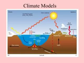
Where from? ( climate model (CM) snow) • CM does mass balance computation for water • Water vapor added to atmosphere at surface • Carried around by convection and winds • Near saturation – makes clouds depending on CCNs • Excess water after saturation removed by precipitation • Phase depends on atmospheric temperature • Ice phase atmospheric water deposited as snow
Snow Mass Budget • Added by atmospheric deposition. • Removed by melting and sublimation. These depend on: • Net radiative balance • (solar and long-wave thermal (LW)) • Micrometeorological delivery of atmosphere sensible heat • Conductive coupling to underlying soil
Climate model simulations • Current standard models are about 1-2 deg resolution and 20-40 layers in vertical. • Integrate many times (ensembles) over hundreds of years. • Can get down to 10s of km for fewer shorter simulations: e.g. 1 annual cycle • Alternate approaches to getting down to 10 km scale (regional climate models or variable mesh) • Cloud resolving scale models – 1 km or less contribute to understanding scaling issues
Examples of snow simulation • CCSM3 – latest NSF/DOE community model. T81 (1.4 deg) atmosphere • Multiple related versions to compare with. • Interactive ocean and sea-ice - • Simulated global land precipitation (averaged by months) falls within existing data sets. • Regionally, precipitation has strong correlations with surface T. • positive for high latitude winter
Land is a complex surface • Consists of many difference surfaces with • Different stores of energy and water • Different radiative and micrometeorological environments. • Separate water and energy balances • Snow component is complex • Spatial variability of cover and depth. • Energy interactions with other surfaces: bare soil and vegetation
Vegetation-snow interactions • Radiative and micrometerological • Micrometerology- canopy generates turbulent mixing that enhances sensible and latent fluxes from snow. • Radiative • longwave exchange (Tempc – Temps) • Solar – shadows subtract solar flux.
Solar radiative forcing of snow by canopy Definitions & notation: assume unit flux normal to surface; snow albedo = α; As = fractional area covered by canopy geometric shadows; Tc = fraction of sunshine transmitted through canopy (sunflecs and diffuse). Canopy cools surface by Qcs: Qcs = As (1.-Tc) (1- α )
Radiative forcing of canopy by snow • Snow heats canopy through the fraction of its reflected radiation that is absorbed by canopy, for single reflection Q sc Qsc =α Acd (1. – Tcd) (1.- Ω) The Acd = 2 As is the fraction of sky shadowed by the canopy from the surface, Tcd is the average transmission of the reflected light, Ω is the canopy ss albedo. • Sum of radiative forcing of snow by canopy (-) and of canopy by snow (+) is the total albedo reduction by the canopy from that of snow alone
What is the net effect? • If lump snow and canopy energy balance together, get net warming: many papers talk about a positive feedback of vegetation on temperature through faster melting of snow. • If just look at solar, however, canopy is cooling the snow. • Net effect depends on net heating by LW and turbulence compared to cooling by solar: may go either way-not adequately treated in current climate models.
Climate model snow albedo in principle α = F (λ, µ, ir, r, s, d, αg, c, g) λ = solar wavelength µ = sun angle projection (cosine) ir= ice index of refraction r = distribution of particle sizes s = distribution of particle shapes d = depth to underlying soil αg = albedo of underlying soil c = concentration/ type of contaminants g = geometry of snow surface
Present snow albedo complexity α = F (λ, µ,r, c) Rationale: • Index of refraction fixed physical constant • Snow depth distribution poorly characterized can assume binary: either deep or no snow • Shapes have been approximated by spheres • Snow geometric effects have been neglected. Further simplification r, c set to values for fresh snow, assumed to correlate an “age” factor
Simple modeling examples of snow radiative forcing by vegetation • Common assumptions made at times: • Leaves have a uniform distribution of orientations or are turbid scatters: makes the optical depth along path of length d simply LAD d /2 where LAD is the local leaf density. • Leaves have low albedo (near black)- true for visible: photons then scatter only once. • Uniform distribution of leaves • Uniform distribution of leaves within a geometric shape (tree or bush)
Uniform leaf distribution snow forcing • Fractional area As =1.0, canopy thickness =d • Optical depth to vertical t= 0.5 d LAD = 0.5 LAI • Transmissivity to radiation incident at angle with cosine µ: • Normalize by divide by snow absorption (1. – α ) • Snow forcing Fs is then simply Fs = (1.- T ) where: T =exp (- t/µ) = 1. – t/µ + 0.5 (t/µ )2 - … (1)
Snow forcing by discrete trees and bushes • Use same LAI – that is per total area – assume sparse enough to ignore mutual shadowing; taking the leaf distributions to be uniform with geometric objects gives local leaf areas as LAI/Ac and their volume averaged optical depths as t/Ac. where Ac is fractional area of object projected into direction of sun (constant for spheres); the geometric shadow As = Ac/µ for sphere object • Tree/bush snow forcing is then : Fs = (Ac/ µ )(1. – T (t/Ac)) (2)
Compare spherical tree versus uniform • Need T to compare – only analytic easy for small since the sphere transmissivity is more complicated than an exponential. By construction of the definition of optical depth, it is T(x) = 1. - x + a x2 +…where a = ? is a constant near unity so Fs = (1. – T) Ac/ µ = t /µ (1 - a / Ac…) (3) To be compared with uniform forcing Eq(1): Fs = t /µ (1- 0.5 t /µ …) (4)
Conclusions • Many subgrid scale processes involving snow that can interact in climate system to produce large scale average effects (i.e. do not average out) • Climate modelers need to identify and include these – not yet very well done. • Vegetation & snow cannot simply average together. Radiative and other interactions complex. • Solar: discrete objects differ from uniform leaves- for same LAI, less radiative effect on snow (at high sun).