Download
1 / 35
350 likes | 436 Vues
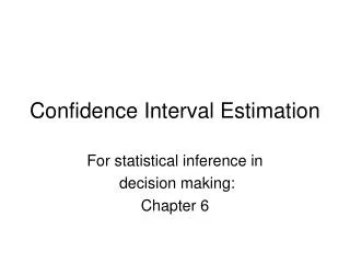
Chapter 23 Confidence Intervals for a Population Mean ; t distributions. t distributions t confidence intervals for a population mean Sample size required to estimate . The Importance of the Central Limit Theorem.

E N D
Chapter 23Confidence Intervals for a Population Mean ; t distributions t distributions t confidence intervals for a population mean Sample size required to estimate
The Importance of the Central Limit Theorem • When we select simple random samples of size n, the sample means we find will vary from sample to sample. We can model the distribution of these sample means with a probability model that is
Since the sampling model for x is the normal model, when we standardize x we get the standard normal z
If is unknown, we probably don’t know either. The sample standard deviation s provides an estimate of the population standard deviation s For a sample of size n,the sample standard deviation s is: n − 1 is the “degrees of freedom.” The value s/√n is called the standard error of x , denoted SE(x).
Standardize using s for • Substitute s (sample standard deviation) for s s s s s s s s Note quite correct Not knowing means using z is no longer correct
t-distributions Suppose that a Simple Random Sample of size n is drawn from a population whose distribution can be approximated by a N(µ, σ) model. When s is known, the sampling model for the mean x is N(m, s/√n), so is approximately Z~N(0,1). When s is estimated from the sample standard deviation s, the sampling model for follows a t distribution with degrees of freedom n − 1. is the 1-sample t statistic
Confidence Interval Estimates • CONFIDENCE INTERVAL for • where: • t = Critical value from t-distribution with n-1 degrees of freedom • = Sample mean • s = Sample standard deviation • n = Sample size • For very small samples (n < 15), the data should follow a Normal model very closely. • For moderate sample sizes (n between 15 and 40), t methods will work well as long as the data are unimodal and reasonably symmetric. • For sample sizes larger than 40, t methods are safe to use unless the data are extremely skewed. If outliers are present, analyses can be performed twice, with the outliers and without.
t distributions • Very similar to z~N(0, 1) • Sometimes called Student’s t distribution; Gossett, brewery employee • Properties: i) symmetric around 0 (like z) ii) degrees of freedom
Z -3 -2 -1 0 1 2 3 -3 -2 -1 0 1 2 3 Student’s t Distribution
Z t -3 -2 -1 0 1 2 3 -3 -2 -1 0 1 2 3 Student’s t Distribution Figure 11.3, Page 372
Degrees of Freedom Z t1 -3 -2 -1 0 1 2 3 -3 -2 -1 0 1 2 3 Student’s t Distribution Figure 11.3, Page 372
Degrees of Freedom Z t1 t7 -3 -2 -1 0 1 2 3 -3 -2 -1 0 1 2 3 Student’s t Distribution Figure 11.3, Page 372
t-Table: text- inside back cover • 90% confidence interval; df = n-1 = 10 0.80 0.95 0.98 0.99 0.90 Degrees of Freedom 1 3.0777 6.314 12.706 31.821 63.657 2 1.8856 2.9200 4.3027 6.9645 9.9250 . . . . . . . . . . . . 10 1.3722 1.8125 2.2281 2.7638 3.1693 . . . . . . . . . . . . 100 1.2901 1.6604 1.9840 2.3642 2.6259 1.282 1.6449 1.9600 2.3263 2.5758
Student’s t Distribution P(t > 1.8125) = .05 P(t < -1.8125) = .05 .90 .05 .05 t10 0 -1.8125 1.8125
Comparing t and z Critical Values Conf. level n = 30 z = 1.645 90% t = 1.6991 z = 1.96 95% t = 2.0452 z = 2.33 98% t = 2.4620 z = 2.58 99% t = 2.7564
Example • An investor is trying to estimate the return on investment in companies that won quality awards last year. • A random sample of 41 such companies is selected, and the return on investment is recorded for each company. The data for the 41 companies have • Construct a 95% confidence interval for the mean return.
Example • Because cardiac deaths increase after heavy snowfalls, a study was conducted to measure the cardiac demands of shoveling snow by hand • The maximum heart rates for 10 adult males were recorded while shoveling snow. The sample mean and sample standard deviation were • Find a 90% CI for the population mean max. heart rate for those who shovel snow.
EXAMPLE: Consumer Protection Agency • Selected random sample of 16 packages of a product whose packages are marked as weighing 1 pound. • From the 16 packages: • a.find a 95% CI for the mean weight of the 1-pound packages • b. should the company’s claim that the mean weight is 1 pound be challenged ?
Chapter 23 Testing Hypotheses about Means 22
Sweetness in cola soft drinks Cola manufacturers want to test how much the sweetness of cola drinks is affected by storage. The sweetness loss due to storage was evaluated by 10 professional tasters by comparing the sweetness before and after storage (a positive value indicates a loss of sweetness): Taster Sweetness loss • 1 2.0 • 2 0.4 • 3 0.7 • 4 2.0 • 5 −0.4 • 6 2.2 • 7 −1.3 • 8 1.2 • 9 1.1 • 10 2.3 We want to test if storage results in a loss of sweetness, thus: H0: m = 0 versus HA: m > 0 where m is the mean sweetness loss due to storage. We also do not know the population parameter s, the standard deviation of the sweetness loss.
The one-sample t-test As in any hypothesis tests, a hypothesis test for requires a few steps: • State the null and alternative hypotheses (H0 versus HA) • Decide on a one-sided or two-sided test • Calculate the test statistic t and determining its degrees of freedom • Find the area under the t distribution with the t-table or technology • State the P-value (or find bounds on the P-value) and interpret the result
The one-sample t-test; hypotheses Step 1: • State the null and alternative hypotheses (H0 versus HA) • Decide on a one-sided or two-sided test H0: m = m0 versus HA: m > m0 (1 –tail test) H0: m = m0 versus HA: m < m0 (1 –tail test) H0: m = m0 versus HA: m ≠ m0 (2 –tail test)
The one-sample t-test; test statistic We perform a hypothesis test with null hypothesis H : = 0 using the test statistic where the standard error of is . When the null hypothesis is true, the test statistic follows a t distribution with n-1 degrees of freedom. We use that model to obtain a P-value.
The one-sample t-test; P-Values Recall: The P-value is the probability, calculated assuming the null hypothesis H0 is true, of observing a value of the test statistic more extreme than the value we actually observed. The calculation of the P-value depends on whether the hypothesis test is 1-tailed (that is, the alternative hypothesis is HA : < 0 or HA : > 0) or 2-tailed (that is, the alternative hypothesis is HA : ≠ 0). 27
P-Values Assume the value of the test statistic t is t0 If HA: > 0, then P-value=P(t > t0) If HA: < 0, then P-value=P(t < t0) If HA: ≠ 0, then P-value=2P(t > |t0|) 28
Sweetening colas (continued) Is there evidence that storage results in sweetness loss in colas?H0: = 0 versus Ha: > 0 (one-sided test) Taster Sweetness loss 1 2.0 2 0.4 3 0.7 4 2.0 5 -0.4 6 2.2 7 -1.3 8 1.2 9 1.1 10 2.3 ___________________________ Average 1.02 Standard deviation 1.196 Degrees of freedom n − 1 = 9 2.2622 < t = 2.70 < 2.8214; thus 0.01 < P-value < 0.025. Since P-value < .05, we reject H0. There is a significant loss of sweetness, on average, following storage.
Finding P-values with Excel TDIST(x, degrees_freedom, tails) TDIST = P(t > x) for a random variable t following the t distribution (x positive).Use it in place of t-table to obtain the P-value. • x is the absolute value of the test statistic. • Deg_freedom is an integer indicating the number of degrees of freedom. • Tails specifies the number of distribution tails to return. If tails = 1, TDIST returns the one-tailed P-value. If tails = 2, TDIST returns the two-tailed P-value.
Sweetness in cola soft drinks(cont.) 2.2622 < t = 2.70 < 2.8214; thus 0.01 < p < 0.025.
The NYC Visitors Bureau claims that the average cost of a hotel room is $168 per night. A random sample of 25 hotels resulted in y = $172.50 and s = $15.40. New York City Hotel Room Costs H0:μ= 168HA:μ ¹168
n = 25; df = 24 New York City Hotel Room Costs t, 24 df H0:μ= 168HA:μ ¹168 .079 .079 0 -1. 46 1. 46 P-value = .158 Do not reject H0: not sufficient evidence that true mean cost is different than $168
A popcorn maker wants a combination of microwave time and power that delivers high-quality popped corn with less than 10% unpopped kernels, on average. After testing, the research department determines that power 9 at 4 minutes is optimum. The company president tests 8 bags in his office microwave and finds the following percentages of unpopped kernels: 7, 13.2, 10, 6, 7.8, 2.8, 2.2, 5.2. Do the data provide evidence that the mean percentage of unpopped kernels is less than 10%? Microwave Popcorn H0:μ= 10 HA:μ <10 where μ is true unknown mean percentage of unpopped kernels
n = 8; df = 7 Microwave Popcorn t, 7 df H0:μ= 10HA:μ <10 .02 0 -2. 51 Exact P-value = .02 Reject H0: there is sufficient evidence that true mean percentage of unpopped kernels is less than 10%