Download
1 / 1
10 likes | 113 Vues
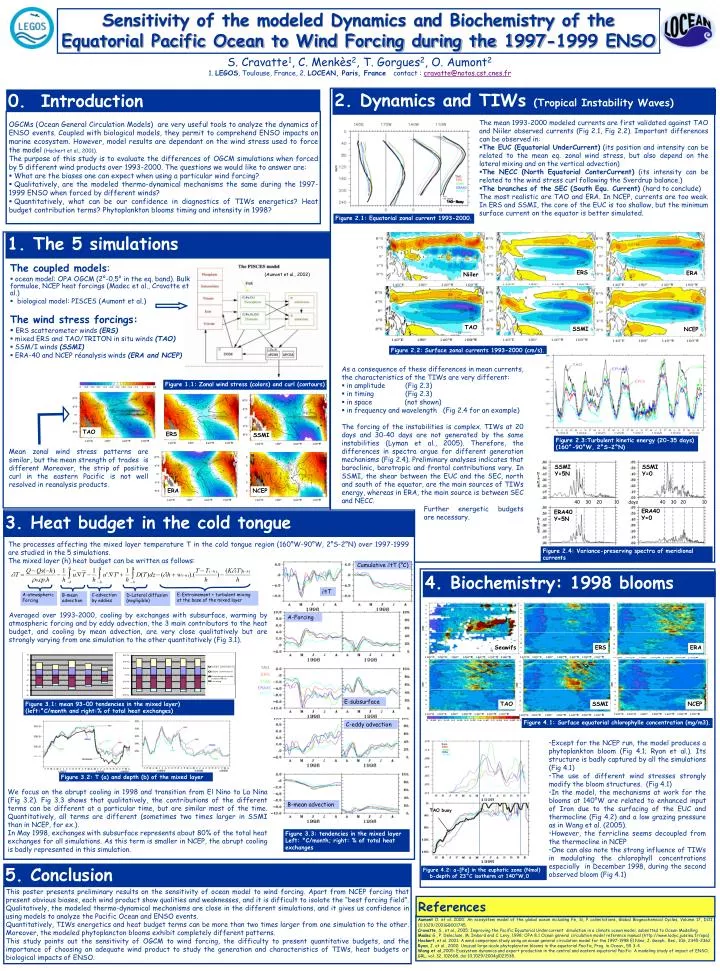
Sensitivity of the modeled Dynamics and Biochemistry of the Equatorial Pacific Ocean to Wind Forcing during the 1997-1999 ENSO. S. Cravatte 1 , C. Menkès 2 , T. Gorgues 2 , O. Aumont 2 1. LEGOS , Toulouse, France, 2. LOCEAN, Paris, France contact : cravatte@notos.cst.cnes.fr.

E N D
Sensitivity of the modeled Dynamics and Biochemistry of the Equatorial Pacific Ocean to Wind Forcing during the 1997-1999 ENSO S. Cravatte1, C. Menkès2, T. Gorgues2, O. Aumont2 1. LEGOS, Toulouse, France, 2. LOCEAN, Paris, France contact : cravatte@notos.cst.cnes.fr 2. Dynamics and TIWs (Tropical Instability Waves) 0. Introduction • The mean 1993-2000 modeled currents are first validated against TAO and Niiler observed currents (Fig 2.1, Fig 2.2). Important differences can be observed in: • The EUC (Equatorial UnderCurrent) (its position and intensity can be related to the mean eq. zonal wind stress, but also depend on the lateral mixing and on the vertical advection) • The NECC (North Equatorial ConterCurrent) (its intensity can be related to the wind stress curl following the Sverdrup balance.) • The branches of the SEC (South Equ. Current) (hard to conclude) • The most realistic are TAO and ERA. In NCEP, currents are too weak. In ERS and SSMI, the core of the EUC is too shallow, but the minimum surface current on the equator is better simulated. • OGCMs (Ocean General Circulation Models) are very useful tools to analyze the dynamics of ENSO events. Coupled with biological models, they permit to comprehend ENSO impacts on marine ecosystem. However, model results are dependant on the wind stress used to force the model (Hackert et al., 2001). • The purpose of this study is to evaluate the differences of OGCM simulations when forced by 5 different wind products over 1993-2000. The questions we would like to answer are: • What are the biases one can expect when using a particular wind forcing? • Qualitatively, are the modeled thermo-dynamical mechanisms the same during the 1997-1999 ENSO when forced by different winds? • Quantitatively, what can be our confidence in diagnostics of TIWs energetics? Heat budget contribution terms? Phytoplankton blooms timing and intensity in 1998? Figure 2.1: Equatorial zonal current 1993-2000. 1. The 5 simulations • The coupled models: • ocean model: OPA OGCM (2°-0.5° in the eq. band). Bulk formulae, NCEP heat forcings (Madec et al., Cravatte et al.) • biological model: PISCES (Aumont et al.) • The wind stress forcings: • ERS scatterometer winds (ERS) • mixed ERS and TAO/TRITON in situ winds (TAO) • SSM/I winds (SSMI) • ERA-40 and NCEP réanalysis winds (ERA and NCEP) (Aumont et al., 2002) Figure 2.2: Surface zonal currents 1993-2000 (cm/s). ERS ERA Niiler • As a consequence of these differences in mean currents, the characteristics of the TIWs are very different: • in amplitude (Fig 2.3) • in timing (Fig 2.3) • in space (not shown) • in frequency and wavelength (Fig 2.4 for an example) The forcing of the instabilities is complex. TIWs at 20 days and 30-40 days are not generated by the same instabilities (Lyman et al., 2005). Therefore, the differences in spectra argue for different generation mechanisms (Fig 2.4). Preliminary analyses indicates that baroclinic, barotropic and frontal contributions vary. In SSMI, the shear between the EUC and the SEC, north and south of the equator, are the main sources of TIWs energy, whereas in ERA, the main source is between SEC and NECC. Further energetic budgets are necessary. Figure 1.1: Zonal wind stress (colors) and curl (contours) TAO SSMI NCEP Figure 2.3:Turbulent kinetic energy (20-35 days) (160°-90°W, 2°S-2°N) ERS Mean zonal wind stress patterns are similar, but the mean strength of trades is different Moreover, the strip of positive curl in the eastern Pacific is not well resolved in reanalysis products. SSMI 40 30 20 10 days 40 30 20 10 ERA NCEP TAO 3. Heat budget in the cold tongue The processes affecting the mixed layer temperature T in the cold tongue region (160°W-90°W, 2°S-2°N) over 1997-1999 are studied in the 5 simulations. The mixed layer (h) heat budget can be written as follows: SSMI Y=5N SSMI Y=0 Figure 2.4: Variance-preserving spectra of meridional currents Cumulative tT (°C) 4. Biochemistry: 1998 blooms tT ERA40 Y=0 ERA40 Y=5N E-Entrainement + turbulent mixing at the base of the mixed layer A-atmospheric Forcing C-advection by eddies B-mean advection D-Lateral diffusion (negligible) A-Forcing Averaged over 1993-2000, cooling by exchanges with subsurface, warming by atmospheric forcing and by eddy advection, the 3 main contributors to the heat budget, and cooling by mean advection, are very close qualitatively but are strongly varying from one simulation to the other quantitatively (Fig 3.1). Seawifs ERS ERA E-subsurface TAO SSMI NCEP Figure 3.1: mean 93-00 tendencies in the mixed layer) (left:°C/month and right:% of total heat exchanges) C-eddy advection Figure 4.1: Surface equatorial chlorophylle concentration (mg/m3). • Except for the NCEP run, the model produces a phytoplankton bloom (Fig 4.1; Ryan et al.). Its structure is badly captured by all the simulations (Fig 4.1) • The use of different wind stresses strongly modify the bloom structures. (Fig 4.1) • In the model, the mechanisms at work for the blooms at 140°W are related to enhanced input of Iron due to the surfacing of the EUC and thermocline (Fig 4.2) and a low grazing pressure as in Wang et al. (2005). • However, the ferricline seems decoupled from the thermocline in NCEP • One can also note the strong influence of TIWs in modulating the chlorophyll concentrations especially in December 1998, during the second observed bloom (Fig 4.1) Figure 3.2: T (a) and depth (b) of the mixed layer We focus on the abrupt cooling in 1998 and transition from El Nino to La Nina (Fig 3.2). Fig 3.3 shows that qualitatively, the contributions of the different terms can be different at a particular time, but are similar most of the time. Quantitatively, all terms are different (sometimes two times larger in SSMI than in NCEP, for ex.). In May 1998, exchanges with subsurface represents about 80% of the total heat exchanges for all simulations. As this term is smaller in NCEP, the abrupt cooling is badly represented in this simulation. B-mean advection TAO buoy Figure 3.3: tendencies in the mixed layer Left: °C/month; right: % of total heat exchanges 5. Conclusion Figure 4.2: a-[Fe] in the euphotic zone (Nmol) b-depth of 23°C isotherm at 140°W,0 This poster presents preliminary results on the sensitivity of ocean model to wind forcing. Apart from NCEP forcing that present obvious biases, each wind product show qualities and weaknesses, and it is difficult to isolate the “best forcing field”. Qualitatively, the modeled thermo-dynamical mechanisms are close in the different simulations, and it gives us confidence in using models to analyze the Pacific Ocean and ENSO events. Quantitatively, TIWs energetics and heat budget terms can be more than two times larger from one simulation to the other. Moreover, the modeled phytoplancton blooms exhibit completely different patterns. This study points out the sensitivity of OGCM to wind forcing, the difficulty to present quantitative budgets, and the importance of choosing an adequate wind product to study the generation and characteristics of TIWs, heat budgets or biological impacts of ENSO. References Aumont O. et al. 2005: An ecosystem model of the global ocean including Fe, Si, P colimitations, Global Biogeochemical Cycles, Volume 17, DOI 10.1029/2001GB001745. Cravatte, S., et al., 2005: Improving the Pacific Equatorial Undercurrent simulation in a climate ocean model, submitted to Ocean Modelling. Madec G., P. Delecluse, M. Imbard and C. Levy, 1998: OPA 8.1 Ocean general circulation model reference manual (http://www.lodyc.jussieu.fr/opa) Hackert, et al. 2001: A wind comparison study using an ocean general circulation model for the 1997-1998 El Nino, J. Geoph.. Res., 106, 2345-2362 Ryan, J. et al., 2002: Unusual large-scale phytoplancton blooms in the equatorial Pacific, Prog. in Ocean., 55 3-4. Wang et al.,2005: Ecosystem dynamics and export production in the central and eastern equatorial Pacific: A modeling study of impact of ENSO, GRL, vol. 32, l02608, doi:10.1029/2004gl021538.